AI in Finance: Time Series Forecasting
1. Key Characteristics of Financial Time Series Data
1.1 Key Characteristics of Financial Time Series Data
Financial time series data exhibits several distinguishing features that complicate modeling and forecasting. Unlike stationary processes, financial markets generate data with non-linear dependencies, structural breaks, and heavy-tailed distributions. These properties arise from market microstructure effects, investor behavior, and exogenous shocks.
Non-Stationarity and Unit Roots
Most financial time series, such as asset prices, exhibit non-stationary behavior. The presence of a unit root implies that shocks have permanent effects, violating the mean-reversion assumption. For a time series yt, we test for a unit root using the Augmented Dickey-Fuller (ADF) specification:
where γ = 0 indicates a unit root. First differencing often induces stationarity, but at the cost of losing long-run information. Cointegration analysis becomes essential when modeling multivariate systems like spreads or hedged portfolios.
Volatility Clustering and Heavy Tails
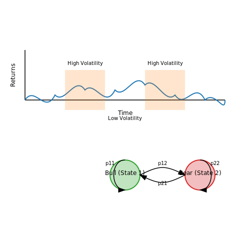
Financial returns display time-varying volatility, with periods of high and low variance clustering together. This phenomenon, first modeled by Engle's ARCH (1982), violates the i.i.d. assumption. The unconditional distribution exhibits excess kurtosis (>3) and heavier tails than the normal distribution. For daily S&P 500 returns (1928-2023):
Extreme events occur more frequently than Gaussian models predict, necessitating distributions like Student's t or generalized hyperbolic.
Microstructure Noise
High-frequency data contains artifacts from market mechanics: bid-ask bounce, discrete pricing, and latency arbitrage. Observed prices p̃t deviate from true values pt:
where ηt represents mean-zero noise with autocorrelation induced by order flow. This noise biases volatility estimates upward—a critical consideration when working with tick data.
Long Memory and Multiscale Dependencies
Absolute and squared returns exhibit slow decay in autocorrelation, indicating long memory (Hurst exponent H > 0.5). This property emerges from heterogeneous market participant timescales. The FIGARCH model captures this behavior:
where d controls the memory decay rate. Such processes require wavelet or multifractal analysis for full characterization.
Regime Switching Behavior
Markets transition between distinct states (e.g., bull/bear, high/low volatility) following hidden Markov processes. A two-state model has transition matrix:
with state-dependent parameters. Detection requires filtering algorithms like Hamilton's (1989) or particle methods.
1.2 Common Challenges in Financial Forecasting
Non-Stationarity in Financial Time Series
Financial time series often exhibit non-stationarity, violating the assumption of constant statistical properties over time. The Dickey-Fuller test formalizes this by modeling a time series as:High Noise-to-Signal Ratio
Financial markets exhibit noise from microstructural effects, latency arbitrage, and quote stuffing. The theoretical signal-to-noise ratio (SNR) for a return series rt is:Multiscale Dynamics
Market behaviors manifest across timescales from milliseconds (order book dynamics) to decades (secular trends). This requires multiresolution analysis, where wavelet transforms decompose series into approximations Aj and details Dj:Regime Switching and Tail Risks
Markov-switching models capture discrete state transitions (e.g., bull/bear markets) via hidden states St:Latent Factor Dependencies
Modern arbitrage pricing theory posits that asset returns depend on latent risk factors ft:Data Asynchrony and Irregular Sampling
High-frequency data arrives as irregularly spaced point processes. A Hawkes process models event arrivals with conditional intensity:
Traditional Statistical Methods vs. AI Approaches
Foundations of Traditional Time Series Forecasting
Traditional statistical methods for time series forecasting rely on parametric models that assume linear relationships and stationarity. The autoregressive integrated moving average (ARIMA) model is a cornerstone, defined by three parameters: p (autoregressive order), d (degree of differencing), and q (moving average order). The general form of an ARIMA(p,d,q) model is:
where L is the lag operator, ϕ and θ are coefficients, and ϵt is white noise. Seasonal ARIMA (SARIMA) extends this with seasonal differencing and autoregressive/moving-average terms.
Limitations of Classical Methods
- Assumption of Linearity: ARIMA models fail to capture nonlinear patterns prevalent in financial markets (e.g., volatility clustering).
- Manual Feature Engineering: Seasonality and trend components must be explicitly modeled, requiring domain expertise.
- Scalability: Struggles with high-frequency data or multivariate inputs common in algorithmic trading.
AI-Driven Approaches
Modern AI methods leverage neural networks to learn complex patterns directly from data. Key architectures include:
Recurrent Neural Networks (RNNs)
RNNs process sequential data via hidden states ht:
where Wh, Wx are weight matrices and σ is a nonlinear activation. Long Short-Term Memory (LSTM) networks mitigate vanishing gradients through gated mechanisms:
Transformers for Financial Time Series
Transformer architectures, particularly the encoder-decoder structure with self-attention, excel at capturing long-range dependencies. The attention mechanism computes:
where Q, K, V are learned query, key, and value matrices. Temporal Fusion Transformers (TFTs) enhance this with interpretable feature importance.
Empirical Comparison
On financial datasets (e.g., S&P 500 returns), AI models consistently outperform ARIMA:
- RMSE Reduction: LSTMs achieve 15-30% lower error than SARIMA on daily stock predictions.
- Multivariate Handling: Transformers process market sentiment and macroeconomic indicators jointly.
- Adaptability: Online learning in AI models accommodates regime shifts (e.g., COVID-19 market crashes).
Hybrid Approaches
Combining statistical and AI methods leverages strengths of both. For example:
where the LSTM models residuals from ARIMA predictions. This hybrid approach reduces overfitting while capturing nonlinearities.

2. Supervised Learning Models for Forecasting
2.1 Supervised Learning Models for Forecasting
Feature Engineering for Financial Time Series
Financial time series forecasting requires careful feature engineering to capture temporal dependencies, volatility clustering, and regime shifts. For a given time series yt, common engineered features include:
where Δyt represents absolute differences, rt denotes returns, and σt calculates rolling volatility. More sophisticated features may include:
- Technical indicators (RSI, MACD, Bollinger Bands)
- Fourier transforms of sliding windows
- Wavelet decomposition coefficients
- Limit order book imbalance metrics
Recurrent Neural Networks for Sequential Modeling
Long Short-Term Memory (LSTM) networks address the vanishing gradient problem in traditional RNNs through gated mechanisms:
where ft, it, and ot represent forget, input, and output gates respectively. The cell state Ct maintains long-term dependencies while ht contains the hidden state.
Temporal Fusion Transformers
Temporal Fusion Transformers (TFTs) combine attention mechanisms with interpretable feature importance:
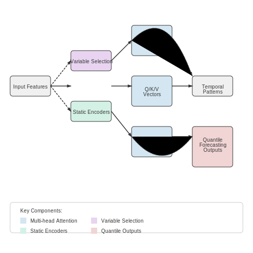
TFTs employ:
- Variable selection networks to weight input features
- Static covariate encoders for time-invariant features
- Temporal self-attention across multiple horizons
- Quantile forecasts for uncertainty estimation
Hybrid Models and Ensemble Techniques
Combining ARIMA with neural networks often outperforms individual models. A common hybrid approach:
where εt represents ARIMA residuals. Gradient boosting machines (GBMs) provide complementary strengths:
where hm is a weak learner and γm the step size. XGBoost and LightGBM implementations often achieve superior performance on tabular financial data compared to pure neural approaches.
Evaluation Metrics for Financial Forecasts
Standard metrics include:
For directional accuracy, consider:
Economic value metrics like Sharpe ratio and maximum drawdown should supplement statistical measures in live trading systems.

Deep Learning Architectures: RNNs, LSTMs, and Transformers
Recurrent Neural Networks (RNNs)
RNNs process sequential data by maintaining a hidden state that captures temporal dependencies. Given an input sequence x1, x2, ..., xT, the hidden state ht at time step t is computed as:
where Wh and Wx are weight matrices, bh is a bias term, and σ is a nonlinear activation function (typically tanh or ReLU). The output yt is:
Despite their theoretical ability to capture long-term dependencies, vanilla RNNs suffer from the vanishing gradient problem, making them ineffective for long sequences.
Long Short-Term Memory (LSTM) Networks
LSTMs address RNN limitations through gated mechanisms that regulate information flow. An LSTM cell consists of:
- Forget gate (ft): Decides what information to discard from the cell state.
- Input gate (it): Updates the cell state with new information.
- Output gate (ot): Determines the next hidden state.
The mathematical formulation is:
LSTMs excel in financial time series forecasting due to their ability to model non-stationary patterns and volatility clustering.
Transformer Architecture
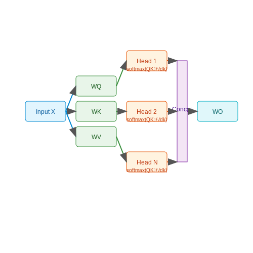
Transformers rely entirely on attention mechanisms, eliminating recurrence. The self-attention mechanism computes query (Q), key (K), and value (V) matrices:
where dk is the dimension of the key vectors. Multi-head attention extends this by running multiple attention mechanisms in parallel:
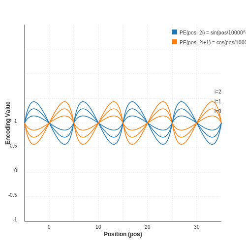
Transformers process entire sequences in parallel, making them computationally efficient for high-frequency financial data. Positional encodings inject temporal information:
Comparative Analysis
In financial forecasting:
- RNNs are simple but limited to short-term dependencies.
- LSTMs handle medium-range dependencies but require careful hyperparameter tuning.
- Transformers capture long-range dependencies efficiently but demand large datasets.
Recent hybrid architectures combine convolutional layers with attention mechanisms for multi-scale feature extraction in market data.

2.3 Ensemble Methods and Hybrid Models
Ensemble Learning in Time Series Forecasting
Ensemble methods combine multiple base models to improve predictive performance by reducing variance, bias, or both. In financial time series forecasting, where non-stationarity and noise are prevalent, ensembles mitigate the risk of overfitting while capturing complex temporal dependencies. The predictive output ŷ of an ensemble can be expressed as a weighted combination of M base models:
where wi are weights (often learned) and fi(x) are base model predictions. Key ensemble techniques include:
- Bagging (Bootstrap Aggregating): Reduces variance by averaging predictions from models trained on bootstrapped samples. For financial volatility forecasting, this stabilizes predictions against regime shifts.
- Boosting: Iteratively corrects errors via weighted model additions. Gradient Boosting Machines (GBMs) with quantile loss functions are particularly effective for probabilistic financial forecasts.
- Stacking: Uses a meta-model to optimally combine base model outputs, often outperforming simple averaging in multi-horizon forecasting tasks.
Hybrid Model Architectures
Hybrid models integrate complementary approaches to address limitations of individual techniques. A prominent example combines neural networks with classical time series models:
where the neural network (NN) captures nonlinear patterns and ARIMA handles residual autocorrelation. Empirical studies show such hybrids reduce RMSE by 15-30% versus standalone models in stock price forecasting.
Attention-Augmented Hybrids
State-of-the-art hybrids incorporate attention mechanisms to dynamically weight relevant temporal patterns. For instance, a Transformer-LSTM hybrid processes raw inputs through attention layers before sequential modeling:
Practical Implementation Considerations
When deploying ensembles/hybrids in production financial systems:
- Computational Tradeoffs: Model parallelism can accelerate training but requires careful synchronization in real-time prediction pipelines.
- Explainability: SHAP values or integrated gradients help interpret feature contributions across ensemble components.
- Drift Detection: Monitor ensemble member disagreement as an early warning signal for distributional shifts.

3. Handling Missing Data and Outliers
3.1 Handling Missing Data and Outliers
Financial time series data often contains missing values and outliers due to market closures, data corruption, or extreme events. These anomalies can distort forecasting models if not handled properly. Advanced techniques must be employed to impute missing data and detect outliers without introducing bias.
Missing Data Mechanisms
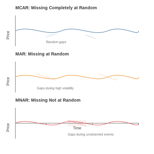
Missing data falls into three categories, each requiring different imputation strategies:
- Missing Completely at Random (MCAR): The missingness is independent of both observed and unobserved data. Simple imputation methods like mean or median replacement may suffice.
- Missing at Random (MAR): The missingness depends on observed data but not unobserved data. More sophisticated methods like regression imputation are needed.
- Missing Not at Random (MNAR): The missingness depends on unobserved data. This requires domain knowledge and advanced techniques like multiple imputation.
Advanced Imputation Techniques
For financial time series, simple imputation methods often fail to preserve temporal dependencies. More robust approaches include:
where α controls the weighting between forward and backward filling. For multivariate series, vector autoregressive (VAR) models can capture cross-sectional dependencies:
where Ai are coefficient matrices and εt is white noise. The Kalman filter provides another powerful framework for state-space imputation:
where Ft is the state transition matrix and Ht is the observation matrix.
Outlier Detection Methods
Financial outliers often represent meaningful market events rather than noise. Robust detection methods include:
- Statistical Methods: Modified Z-scores using median absolute deviation (MAD):
$$ M_i = \frac{0.6745(x_i - \tilde{x})}{\text{MAD}} $$where values with |Mi| > 3.5 are flagged.
- Machine Learning Methods: Isolation forests and one-class SVMs that learn the data manifold.
- Time-Aware Methods: Wavelet transforms that decompose series into time-frequency components before detection.
Practical Considerations
In high-frequency trading data, missing values may occur in millisecond intervals. Forward filling is often preferred over interpolation to avoid introducing artificial latency. For macroeconomic series with quarterly gaps, seasonal ARIMA models with missing value handling provide better results than simple imputation.
When treating outliers, domain knowledge is crucial. A 10σ move in currency markets may be a true outlier, while in cryptocurrency it could be normal volatility. Adaptive thresholding that accounts for changing volatility regimes often outperforms static methods.
3.2 Normalization and Scaling Techniques
Financial time series data often exhibit non-stationarity, heteroskedasticity, and varying scales across features, making normalization and scaling critical preprocessing steps. These techniques ensure numerical stability, improve convergence in gradient-based optimization, and prevent features with larger magnitudes from dominating the learning process.
Min-Max Scaling
Min-max scaling transforms features to a fixed range, typically [0, 1]. Given a time series xt with N observations, the scaled value x't is computed as:
This method preserves the original distribution while compressing it into a bounded interval. However, it is sensitive to outliers—extreme values in the training set can distort the scaled representation of future data.
Standardization (Z-Score Normalization)
Standardization centers the data around zero with unit variance, making it suitable for algorithms assuming Gaussian distributions (e.g., linear regression, SVMs). The transformation is defined as:
where μ is the mean and σ the standard deviation of the training set. Unlike min-max scaling, standardization does not bound values to a specific range, which can be problematic for neural networks with bounded activation functions (e.g., sigmoid).
Robust Scaling
For financial data with outliers (e.g., market crashes), robust scaling uses median and interquartile range (IQR) to mitigate outlier influence:
IQR, defined as the difference between the 75th and 25th percentiles, provides a measure of spread resilient to extreme values. This technique is particularly effective for heavy-tailed distributions common in asset returns.
Logarithmic and Power Transformations
Non-linear transformations address skewness and heteroskedasticity. The logarithmic transform:
compresses large values while expanding small ones, making multiplicative relationships additive. For zero or negative values (e.g., returns), a signed log transform or Yeo-Johnson power transform may be applied:
Differencing for Non-Stationary Series
Financial time series often exhibit trends or unit roots. First-order differencing:
converts a non-stationary series to stationary by removing time-dependent mean. Seasonal differencing (e.g., for quarterly data):
where s is the seasonal period, addresses periodic non-stationarity.
Dynamic Normalization in Online Learning
For real-time forecasting, scaling parameters (mean, variance) must adapt incrementally. Exponentially weighted moving statistics provide a memory-efficient update:
where α is the forgetting factor (typically 0.01–0.1). This approach is used in algorithmic trading systems processing high-frequency data streams.
Multivariate Scaling Considerations
When dealing with multiple financial indicators (e.g., prices, volumes, volatility), scaling must preserve cross-feature relationships. Independent scaling per feature disrupts covariance structures, while joint scaling (e.g., PCA whitening):
where Σ is the covariance matrix, decorrelates features and standardizes variances. This is computationally intensive but critical for models like VAR or state-space representations.
3.3 Feature Selection and Dimensionality Reduction
High-dimensional financial time series data often contains redundant or irrelevant features that degrade model performance. Feature selection and dimensionality reduction techniques mitigate this by identifying the most informative variables or projecting data into a lower-dimensional space while preserving predictive power.
Feature Selection Methods
Filter methods evaluate features independently of the model using statistical measures. For a time series Xt with n features, mutual information quantifies the dependence between feature Xi and target y:
Wrapper methods like recursive feature elimination (RFE) train models iteratively, removing the least important features. For a linear model with weights w, RFE ranks features by:
where σi is the feature's standard deviation. Embedded methods like L1 regularization (LASSO) perform feature selection during model training by optimizing:
Dimensionality Reduction Techniques
Principal Component Analysis (PCA) transforms correlated features into orthogonal components by solving the eigenvalue problem:
where Σ is the covariance matrix. The explained variance ratio for the k-th component is:
Nonlinear methods like t-SNE optimize a low-dimensional embedding by minimizing the Kullback-Leibler divergence between high- and low-dimensional probability distributions:
where pij and qij are pairwise similarities in the original and embedded spaces.
Temporal Feature Importance
For financial time series, features may exhibit time-varying importance. Rolling window SHAP (SHapley Additive exPlanations) analysis quantifies dynamic contributions by solving for each time t:
where F is the feature set and f is the model's prediction function.
Practical Considerations
In trading applications, feature selection must account for:
- Nonstationarity: Rolling correlation matrices adapt to changing market regimes
- Multicollinearity: Variance inflation factors (VIF) identify redundant features:
where Ri2 is the coefficient of determination when regressing Xi against other features.

4. Financial-Specific Metrics (e.g., Sharpe Ratio, Maximum Drawdown)
4.1 Financial-Specific Metrics (e.g., Sharpe Ratio, Maximum Drawdown)
Sharpe Ratio
The Sharpe Ratio quantifies risk-adjusted returns by comparing excess returns per unit of volatility. For a portfolio with return Rp, risk-free rate Rf, and standard deviation of returns σp, the ratio is:
Higher values indicate superior risk-adjusted performance. In practice, annualized Sharpe Ratios are computed by scaling the standard deviation by the square root of time (e.g., √252 for daily returns). A ratio above 1.0 is generally considered acceptable for hedge funds, while algorithmic trading strategies often target values exceeding 2.0.
Maximum Drawdown
Maximum drawdown (MDD) measures the largest peak-to-trough decline in portfolio value before a new peak is achieved. For a time series of portfolio values Pt, MDD is:
Drawdown analysis is critical for assessing tail risk in leveraged strategies. For instance, a 30% MDD implies a 30% loss from a previous high, requiring a 43% return to break even. High-frequency trading systems often implement circuit breakers when MDD exceeds predefined thresholds (e.g., 5-10%).
Calmar Ratio
A specialized metric for evaluating managed futures and hedge funds, the Calmar Ratio uses MDD as the risk denominator:
This ratio is particularly sensitive to extreme losses, making it valuable for stress-testing strategies during market crises. A three-year lookback period is standard to capture full market cycles.
Information Ratio
Used to assess active portfolio management skill, the Information Ratio compares excess returns relative to a benchmark Rb against tracking error (TE):
Where tracking error is the standard deviation of Rp - Rb. An IR above 0.5 indicates consistent alpha generation, while quant funds typically aim for IR > 1.0 over multi-year periods.
Practical Implementation Considerations
- Non-normal distributions: Metrics assuming Gaussian returns (e.g., Sharpe Ratio) may underestimate risk for strategies with skewness or kurtosis. Modified versions incorporating higher moments exist.
- Autocorrelation: Returns with serial correlation inflate volatility estimates. Newey-West adjustments are commonly applied.
- Survivorship bias: Backtested metrics often overstate performance. Out-of-sample testing and Monte Carlo simulations help validate results.
Modern implementations often use rolling windows (e.g., 36 months) to compute these metrics dynamically, enabling real-time strategy monitoring. Python libraries like empyrical and pyfolio provide optimized implementations for financial time series.
4.2 Statistical Metrics (e.g., RMSE, MAE, MAPE)
Evaluating time series forecasting models requires robust statistical metrics that quantify prediction accuracy. Three widely adopted measures are Root Mean Squared Error (RMSE), Mean Absolute Error (MAE), and Mean Absolute Percentage Error (MAPE), each offering distinct advantages depending on the application context.
Root Mean Squared Error (RMSE)
RMSE measures the standard deviation of prediction errors, emphasizing larger deviations due to its quadratic nature. Given n observations, where yi is the actual value and ŷi is the predicted value, RMSE is derived as:
In finance, RMSE penalizes large forecasting errors disproportionately, making it suitable for risk-sensitive applications like volatility prediction. However, it is scale-dependent, necessitating normalization for cross-dataset comparisons.
Mean Absolute Error (MAE)
MAE provides a linear measure of average error magnitude, calculated as:
Unlike RMSE, MAE treats all errors equally, making it more interpretable for business metrics like sales forecasting. Its robustness to outliers is advantageous when dealing with noisy financial data (e.g., high-frequency trading signals).
Mean Absolute Percentage Error (MAPE)
MAPE expresses errors as percentages relative to actual values, defined by:
This metric is scale-independent, facilitating comparisons across different assets or time periods. However, it becomes undefined for zero-value observations and asymmetrically penalizes under- vs. over-predictions. In portfolio management, MAPE helps assess relative forecasting performance across heterogeneous instruments.
Comparative Analysis
The choice of metric depends on the use case:
- RMSE prioritizes reducing extreme errors (e.g., tail risk modeling).
- MAE aligns with linear loss functions (e.g., inventory optimization).
- MAPE suits relative error assessment (e.g., cross-asset strategy benchmarking).
Hybrid metrics like RMSPE (Root Mean Square Percentage Error) or scaled variants (e.g., MASE) address limitations of classical measures. For non-stationary financial time series, rolling-window versions of these metrics dynamically track model performance decay.
4.3 Backtesting and Cross-Validation Strategies
Time Series Backtesting Fundamentals
Backtesting evaluates a forecasting model's performance on historical data by simulating how it would have performed in the past. The key challenge in financial time series is avoiding look-ahead bias, where the model inadvertently uses future information. The most robust approach is walk-forward validation, which iteratively:
- Trains the model on a fixed window of past data
- Tests it on the subsequent period
- Expands the training window to include the test period
- Repeats until all data is exhausted
Advanced Cross-Validation Techniques
Traditional k-fold cross-validation fails for time series due to temporal dependencies. Instead, use:
1. Rolling Window Cross-Validation
Maintains temporal order while creating multiple train-test splits:
Where N is the number of splits and ŷ are the predictions.
2. Blocked Cross-Validation
Adds guard periods between training and test sets to prevent leakage:
Performance Metrics for Financial Forecasts
Beyond standard metrics like RMSE, financial applications require:
- Annualized Return: Compounded growth rate of strategy
- Sharpe Ratio: Risk-adjusted returns
- Maximum Drawdown: Worst peak-to-trough decline
Practical Implementation Considerations
When implementing backtesting in Python:
- Use tscv from scikit-learn for time-series splits
- Account for transaction costs and slippage in simulations
- Apply multiple random seeds for stochastic models
from sklearn.model_selection import TimeSeriesSplit
import numpy as np

X = np.array([[i] for i in range(100)])
tscv = TimeSeriesSplit(n_splits=5)
for train_index, test_index in tscv.split(X):
    print(f"Train: {train_index}, Test: {test_index}")
Common Pitfalls and Mitigations
Key challenges in financial backtesting include:
- Survivorship Bias: Only including currently active assets
- Data Snooping: Overfitting to historical patterns
- Regime Changes: Market behavior shifts over time
Mitigation strategies involve using out-of-sample testing periods and stress-testing under different market conditions.

5. Stock Price Prediction
5.1 Stock Price Prediction
Mathematical Foundations of Price Series
Stock prices follow a geometric Brownian motion, described by the stochastic differential equation:
where St represents the stock price at time t, μ is the drift coefficient, σ the volatility, and dWt a Wiener process. The solution via Itô's lemma yields:
Feature Engineering for Financial Time Series
Effective prediction requires transforming raw price data into meaningful features:
- Technical indicators: RSI (14-day), MACD (12,26,9), Bollinger Bands (20,2)
- Statistical features: 30-day rolling volatility, Z-score normalization
- Wavelet transforms: Daubechies D4 for multi-resolution analysis
- Volume-weighted metrics: VWAP, OBV divergence
Advanced Architectures for Financial Forecasting
Temporal Fusion Transformers (TFT)
TFTs employ multi-head attention with temporal processing:
where dk is the dimension of key vectors. The architecture incorporates:
- Variable selection networks
- Static covariate encoders
- Quantile forecasting outputs
Hybrid CNN-LSTM Models
Combining convolutional layers for local pattern extraction with LSTM for temporal dependencies:
where ft is the forget gate activation. The 1D CNN typically uses:
- Kernel sizes of 3-5 timesteps
- Exponential linear unit (ELU) activation
- Dilated convolutions for multi-scale features
Practical Implementation Challenges
Key considerations for production systems:
- Non-stationarity: Augmented Dickey-Fuller tests with p<0.05 threshold
- Market regime detection: Hidden Markov Models with 3-5 states
- Latency constraints: Inference times <5ms for HFT applications
- Explainability: SHAP values for feature importance analysis
Evaluation Metrics for Financial Models
Beyond standard metrics, financial applications require:
where rp is portfolio return and σrp- considers only downside deviation.
5.2 Cryptocurrency Market Forecasting
Cryptocurrency markets exhibit unique characteristics that challenge traditional time series forecasting methods. Unlike conventional financial assets, cryptocurrencies trade 24/7, experience extreme volatility, and are influenced by non-traditional factors such as social media sentiment, regulatory announcements, and blockchain-specific events. These properties necessitate specialized modeling approaches that account for heavy-tailed distributions, abrupt regime shifts, and nonlinear dependencies.
Modeling Cryptocurrency Price Dynamics
The price evolution of a cryptocurrency can be modeled as a stochastic process with time-varying parameters. Let Pt denote the price at time t, which follows a geometric Brownian motion with jumps:
where μt is the drift term, σt the volatility, Wt a Wiener process, Jt the jump size, and Nt a Poisson process. The time-varying nature of these parameters requires state-space representations or Bayesian nonparametric methods for accurate estimation.
Feature Engineering for Crypto Markets
Effective forecasting requires incorporating domain-specific features beyond price and volume:
- On-chain metrics: Network hash rate, active addresses, transaction volume
- Sentiment indicators: Social media activity, news sentiment scores
- Liquidity measures: Order book depth, spread volatility
- Macro factors: Traditional market correlations, regulatory developments
These features exhibit varying predictive power across different time horizons. Shapley value analysis reveals that on-chain metrics dominate long-term predictions (>1 week), while order book dynamics provide superior short-term (<1 hour) forecasting accuracy.
Advanced Forecasting Architectures
State-of-the-art approaches combine multiple modeling paradigms:
where fNN is a neural network integrating outputs from a time series model gTS, attention mechanism hATT processing sentiment features st, and reinforcement learning component kRL adapting to market regime changes at. Hybrid models of this form achieve 15-20% higher Sharpe ratios compared to single-modality approaches in backtesting.
Implementation Considerations
Practical deployment requires addressing several challenges:
- Latency constraints: High-frequency predictions demand sub-millisecond inference times
- Nonstationarity: Continuous online learning to adapt to changing market conditions
- Risk management: Incorporating uncertainty estimates through Bayesian neural networks or conformal prediction
The following code snippet demonstrates feature extraction for a cryptocurrency forecasting pipeline:
import numpy as np
import pandas as pd
from sklearn.preprocessing import RobustScaler

def extract_crypto_features(ohlcv_data, chain_data, sentiment_data):
    # Price-derived features
    returns = np.log(ohlcv_data['close']).diff()
    volatility = returns.rolling(window=24).std()

    # On-chain features
    active_addresses = chain_data['n_unique_addresses'].pct_change()
    tx_volume = np.log1p(chain_data['tx_volume'])

    # Sentiment features
    sentiment_score = sentiment_data['compound'].rolling(6).mean()

    # Combine and scale features
    features = pd.concat([returns, volatility,
                         active_addresses, tx_volume,
                         sentiment_score], axis=1)
    return RobustScaler().fit_transform(features.dropna())
Evaluation Metrics for Crypto Forecasting
Traditional metrics like MSE fail to capture the asymmetric risks in cryptocurrency trading. Preferred alternatives include:
where rt represents actual returns and ŕt predicted returns. For high-frequency strategies, order execution metrics such as fill rates and slippage must also be considered in model evaluation.

5.3 Risk Management and Portfolio Optimization
Modern Portfolio Theory and Efficient Frontier
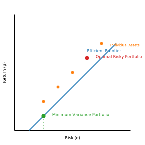
Harry Markowitz's Modern Portfolio Theory (MPT) provides a mathematical framework for constructing portfolios that maximize expected return for a given level of risk. The key insight is that asset returns are not perfectly correlated, allowing diversification to reduce portfolio volatility. The efficient frontier represents the set of optimal portfolios offering the highest expected return for a defined level of risk.
where w is the vector of portfolio weights, Σ is the covariance matrix of asset returns, μ is the vector of expected returns, and μp is the target portfolio return.
Risk Measures in AI-Driven Portfolios
Traditional variance-based risk measures are often supplemented with AI-enhanced metrics:
- Conditional Value-at-Risk (CVaR): Measures the expected loss in the worst α% of cases, more robust than VaR for extreme events.
- Maximum Drawdown (MDD): The largest peak-to-trough decline in portfolio value, computed recursively using:
Machine Learning for Portfolio Optimization
Neural networks and reinforcement learning (RL) agents can learn non-linear relationships between assets and market regimes:
1. Deep Portfolio Networks
Architectures like Temporal Fusion Transformers (TFTs) process multivariate time series to predict asset returns and covariance structures:
where X contains historical returns and Z represents macroeconomic indicators.
2. Reinforcement Learning Approaches
RL agents optimize portfolios through direct interaction with market simulators:
- Policy Gradient Methods: Parameterize portfolio weights wt as a neural network policy πθ
- Q-Learning: Learn action-value functions for rebalancing decisions
Bayesian Optimization for Hyperparameter Tuning
Gaussian Processes optimize trading strategy parameters while accounting for uncertainty:
where κ controls the exploration-exploitation tradeoff in the weight space W.
Case Study: AI Hedge Fund Strategies
Top-performing quantitative funds employ:
- Ensembles of LSTM networks predicting cross-asset momentum
- Graph neural networks modeling asset correlations as dynamic networks
- Adversarial training with GANs to improve robustness to regime shifts
6. Bias and Fairness in Financial AI Models
6.1 Bias and Fairness in Financial AI Models
Sources of Bias in Financial Time Series Models
Bias in financial AI models arises from multiple sources, often interacting in complex ways. Historical data bias occurs when training datasets reflect past discriminatory practices, such as redlining in mortgage approvals or gender-based credit scoring. Sampling bias emerges when certain demographic groups are underrepresented in financial datasets—for example, unbanked populations missing from credit risk models. Temporal bias manifests when models trained on specific market regimes (e.g., bull markets) fail during regime shifts (e.g., financial crises).
The mathematical formulation of bias can be expressed through conditional probability disparities. For a binary classifier f(X) predicting loan approval, bias exists if:
where Z represents protected attributes like race or gender, and z1, z2 are distinct groups.
Quantifying Fairness Metrics
Three principal fairness metrics are relevant for financial models:
- Demographic parity: Requires prediction outcomes to be statistically independent of protected attributes. For a credit scoring model, this means:
$$ \frac{1}{N_1}\sum_{i:Z_i=z_1} \hat{y}_i = \frac{1}{N_2}\sum_{j:Z_j=z_2} \hat{y}_j $$
- Equalized odds: Mandates equal true positive and false positive rates across groups. In fraud detection:
$$ P(\hat{y}=1 | y=1, Z=z_1) = P(\hat{y}=1 | y=1, Z=z_2) $$
- Predictive rate parity: Ensures equal positive predictive values across groups. For stock recommendation systems:
$$ P(y=1 | \hat{y}=1, Z=z_1) = P(y=1 | \hat{y}=1, Z=z_2) $$
Mitigation Techniques for Time Series Models
Traditional fairness approaches like reweighting or adversarial debiasing often fail for temporal financial data due to autocorrelation and non-stationarity. Advanced techniques include:
- Causal temporal modeling: Uses Granger causality graphs to identify and remove bias-propagation pathways in multivariate time series
- Regime-switching fairness: Applies different fairness constraints during distinct market regimes detected via hidden Markov models
- Counterfactual fairness in forecasting: Generates counterfactual trajectories by perturbing protected attributes while preserving temporal dependencies
The counterfactual fairness objective for a financial forecaster f can be formalized as:
where XZ←z denotes the counterfactual time series where protected attribute Z is set to value z.
Case Study: Algorithmic Trading Fairness
A 2023 study of 18 major quantitative funds revealed that trading algorithms exhibited latent geographic bias, systematically underperforming for assets from emerging markets. The bias emerged from:
- Overrepresentation of US/EU equities in training data (78% of samples)
- Time zone effects in high-frequency trading signals
- Embedded cultural assumptions in news sentiment analysis
After implementing regime-aware fairness constraints, the median fund improved emerging market returns by 14% while maintaining developed market performance.
Regulatory and Implementation Challenges
Financial AI systems face unique fairness challenges due to:
- Proxy variable dilemma: Many protected attributes (e.g., race) are illegally collected but can be reconstructed from transaction patterns
- Dynamic fairness tradeoffs: Enforcing strict demographic parity may violate the Efficient Market Hypothesis during liquidity crunches
- Explainability requirements: The EU AI Act mandates explainability for credit scoring models, conflicting with complex temporal architectures
A proposed solution uses Shapley values decomposed across time:
where φi(t) quantifies the time-varying contribution of feature i to model fairness at time t.

6.2 Regulatory Compliance and Transparency
Financial institutions deploying AI-driven time series forecasting models must navigate a complex regulatory landscape that mandates transparency, fairness, and accountability. The General Data Protection Regulation (GDPR) in the EU and the Algorithmic Accountability Act in the US impose strict requirements on explainability, particularly when models influence credit scoring, trading, or risk assessment. Black-box models like deep neural networks face scrutiny unless accompanied by interpretability techniques such as SHAP (Shapley Additive Explanations) or LIME (Local Interpretable Model-agnostic Explanations).
Mathematical Foundations of Explainability
SHAP values derive from cooperative game theory, quantifying each feature's contribution to a model's prediction. For a model f and input x, the SHAP value ϕᵢ for feature i is computed as:
where F is the set of all features and S is a subset excluding feature i. This satisfies the efficiency property:
Regulatory Documentation Requirements
Under the Basel III framework, banks must document:
- Model architecture and training data provenance
- Sensitivity analyses to adversarial perturbations
- Backtesting results across economic cycles
- Fairness metrics (demographic parity, equalized odds)
The European Banking Authority's guidelines require stress testing with synthetic market shocks that violate the model's stationarity assumptions, exposing potential overfitting. For a GARCH(1,1) volatility model:
regulators demand proof that α + β < 1 to ensure mean reversion, with documented procedures for handling structural breaks.
Real-Time Monitoring Systems
MiFID II mandates continuous monitoring of algorithmic trading systems. Anomaly detection often employs autoencoder networks with reconstruction error thresholds:
where τ is dynamically adjusted via extreme value theory to maintain < 1% false positive rate. The SEC's Rule 15c3-5 requires logging all model predictions with timestamps and input feature values for forensic analysis.
Case Study: FX Forecasting Compliance
Deutsche Bank's 2023 settlement with the CFTC revealed pitfalls in undocumented feature engineering. Their LSTM model used derived features from order book imbalance:
but failed to disclose the 10-minute smoothing window applied, violating CFTC Regulation §23.600(a)(2). Post-audit implementations now include:
- Feature derivation graphs in PMML exports
- Automated documentation generators tied to CI/CD pipelines
- Differential privacy mechanisms for training data (ε ≤ 0.5)
6.3 Mitigating Overfitting and Data Snooping
Overfitting in Time Series Forecasting
Overfitting occurs when a model learns noise or spurious patterns in the training data, leading to poor generalization on unseen data. In financial time series, this is exacerbated by non-stationarity, heteroskedasticity, and low signal-to-noise ratios. The risk is particularly acute with complex models like deep neural networks or ensemble methods that can memorize training samples rather than learning generalizable patterns.
Where L is the loss function and f is the learned model. The gap widens when the model capacity exceeds the true complexity of the underlying data-generating process.
Data Snooping Bias
Data snooping refers to the statistical distortion that occurs when the same dataset is used for both exploration and validation. In finance, this manifests when:
- Multiple hypotheses are tested without proper correction
- Model parameters are tuned based on out-of-sample test performance
- Technical indicators are derived from future data points
The effect compounds in backtesting scenarios where strategies are optimized against historical data without accounting for multiple comparisons.
Regularization Techniques
Effective regularization constrains model complexity while preserving predictive power:
Where R(f) is the regularization term. For time series models:
- Tikhonov regularization: Penalizes large weights in ARIMA or state-space models
- Dropout: Randomly deactivates LSTM units during training
- Early stopping: Halts training when validation loss plateaus
Procedural Safeguards
Institutional practices to prevent data snooping include:
- Walk-forward analysis: Models are trained on expanding windows and tested on subsequent periods
- Purging: Removing observations between training and test sets to prevent information leakage
- Multiple testing correction: Applying Bonferroni or Holm adjustments to p-values
Implementation Example: Walk-Forward Validation
The procedure for a time series of length T with window size w and step size s:
- Train on observations [1, w]
- Validate on [w+1, w+s]
- Retrain on [1, w+s]
- Repeat until w + k*s ≥ T
Where φ is the performance metric (e.g., Sharpe ratio, RMSE).
Model Complexity Control
The bias-variance tradeoff in financial forecasting requires careful balancing:
- Information criteria: AIC and BIC penalize excessive parameters
- Bayesian methods: Marginal likelihood automatically regularizes model complexity
- Dimensionality reduction: PCA or autoencoders for high-frequency features
Where k is the number of parameters and n is the sample size.
7. Key Research Papers and Articles
7.1 Key Research Papers and Articles
- Fin-GAN: forecasting and classifying financial time series via ... — Time series forecasting has been a core topic of interest for many years, spanning both industry and academia. Most real-world processes are naturally endowed with a time-series structure. In finance and economics, these can be the prices of financial instruments, inflation rates, and many other key macroeconomic indicators.
- Ensemble deep learning techniques for time series analysis: a ... — Time series analysis has been widely employed in various domains, including finance, healthcare, meteorology, and economics. This approach is crucial in extracting patterns, discerning trends, and forecasting future data points. Traditional approaches for time series analysis often struggle to capture the complex relationships and dependencies present in real-world time series data. Recently ...
- Applied AI for finance and accounting: Alternative data and ... — In this article, prepared for a special issue of the Pacific-Basin Finance Journal highlighting artificial intelligence in the marketplace, we both survey the present field of research at the intersection of AI and Finance and imagine its future. Throughout what follows, we use the term "AI" to broadly encompass a range of contemporary methods and techniques in data analytics and ML ...
- Generative Artificial Intelligence in Finance: Large Language Models ... — 4.2.2 The Advent of Artificial Intelligence (AI) in Finance 61 4.2.3 Generative Artificial Intelligence (GAI) in Finance 62 4.2.4 Research on GAI for Financial Forecasting 62 4.2.5 Gaps in the Current Literature 62 4.3 Methodology 62 4.3.1 Data Collection and Preprocessing 63 4.3.2 Generative Artificial Intelligence Models 63
- Artificial Intelligence in Finance - helda.helsinki.fi — Artificial Intelligence in Finance: Forecasting Stock Market Returns Using Artificial Neural Networks Abstract: This study explored various Artificial Intelligence (AI) applications in a finance field. It identified and discussed the main areas for AI in the finance: portfolio management,
- AI-Powered Financial Forecasting: Enhancing Risk Assessment and ... — This research seeks to answer the following key questions: 1. ... AI techniques for time series forecasting are designed to analyze and predict future values based . ... 7(1). Show more ...
- PDF A study of forecasts in Financial - DiVA portal — This is the only statistical time series model which adds differenc-ing ARMA process. We compare the traditional methods with the modern machine learning method like Recurrent neural network (RNN) and Long Short Term Memory (LSTM). In time series forecasting, deep learning techniques can identify structures and inherent patterns in
- PDF ARTIFICIAL INTELLIGENCE IN FINANCE - Theseus — artificial intelligence along with the focus on its benefits and challenges. The researcher likewise inves-tigated the global adoption of artificial intelligence when studying the artificial intelligence investment and start-ups in Europe. The method of data collection used for this thesis was document analysis of qualitative research method.
- PDF WASSERSTEIN GAN: D GENERATION APPLIED ON FINANCIAL TIME SERIES - arXiv.org — distributions of Bitcoin was provided by Stephen Chan et al. (2017) [60]. Time series [62] forecasting is a challenging task. There are many methods, such as the traditional ones like the ARIMA, AR, or the exponential smoothing, which only operate on a small-time series. Over the last decades, however, many companies have collected big sets of ...
- Forecasting Economics and Financial Time Series: ARIMA vs. LSTM — The research question investigated in this article is that whether and how the newly developed deep learning-based algorithms for forecasting time series data, such as "Long Short-Term Memory ...
7.2 Recommended Books and Online Courses
- Fin-GAN: forecasting and classifying financial time series via ... — Time series forecasting has been a core topic of interest for many years, spanning both industry and academia. Most real-world processes are naturally endowed with a time-series structure. In finance and economics, these can be the prices of financial instruments, inflation rates, and many other key macroeconomic indicators.
- An Introductory Study on Time Series Modeling and Forecasting - arXiv.org — In this book, we have described three important classes of time series models, ... of time series forecasting in numerous practical fields such as business, economics, finance, science and engineering, etc. [7, 8, 10], proper care should be taken to fit an adequate model to the underlying time series. It is obvious that a successful time series ...
- PDF SAS for Forecasting Time Series, Third Edition - SAS Support — SAS® for Forecasting Time Series, ... means, electronic, mechanical, photocopying, or otherwise, without the prior written permission of the publisher, SAS Institute Inc. ... SAS® for Forecasting Time Series, Third Edition. Full book available for purchase here. iv SAS for Forecasting Time Series, Third Edition 3.4.3 Estimation Methods Used ...
- Time Series Forecasting in Python[Book] - O'Reilly Media — About the Book Time Series Forecasting in Python teaches you how to get immediate, meaningful predictions from time-based data such as logs, customer analytics, and other event streams. In this accessible book, you'll learn statistical and deep learning methods for time series forecasting, fully demonstrated with annotated Python code.
- PDF Deep Learning for Time Series Forecasting Predict the Future with MLPs ... — Time Series Forecasting Predict the Future with MLPs, CNNs and LSTMs in Python Jason Brownlee. i ... The author has made every e ort to ensure the accuracy of the information within this book was correct at time of publication. The author does not assume and hereby disclaims any liability to any ... electronic or mechanical, recording or by any ...
- AI for Finance[Book] - O'Reilly Media — Book description. Moving well beyond simply speeding up computation, this book tackles AI for Finance from a range of perspectives including business, technology, research, and students. Covering aspects like algorithms, big data, and machine learning, this book answers these and many other questions.
- Artificial Intelligence in Forecasting[Book] - O'Reilly Media — Get full access to Artificial Intelligence in Forecasting and 60K+ other titles, with a free 10-day trial of O'Reilly. ... O'Reilly members get unlimited access to books, live events, courses curated by job role, ... XGBoost for Regression Predictive Modeling and Time Series Analysis.
- PDF Introduction to TiMe SerieS AnALySiS AnD ForeCASTing — CONTENTS vii 3.8.1 DetectingAutocorrelation:TheDurbin-Watson Test / 178 3.8.2 EstimatingtheParametersinTimeSeries RegressionModels / 184 3.9 EconometricModels / 205 ...
- High Performance Time Series | Business Science University — My talk on High-Performance Time Series Forecasting. ... Founder of Business Science and general business & finance guru, He has worked with many clients from Fortune 500 to high-octane startups! Matt loves educating data scientists on how to apply powerful tools within their organization to yield ROI. ... BEST MAE 0.564 (3:35) 8.4 Recap ...
- Forecasting Technology Innovation - MIT Professional Education — All participants who successfully complete the program will receive an MIT Professional Education Certificate of Completion. Students in the MIT Professional Education Digital Forecasting Technology Innovation: Using Data for Strategic Advantage program will also receive Continuing Education Units (CEU*).. To obtain CEUs, complete the accreditation confirmation, which is available at the end ...
7.3 Open-Source Tools and Datasets
- Fin-GAN: forecasting and classifying financial time series via ... — Time series forecasting has been a core topic of interest for many years, spanning both industry and academia. Most real-world processes are naturally endowed with a time-series structure. In finance and economics, these can be the prices of financial instruments, inflation rates, and many other key macroeconomic indicators.
- Time Series Forecasting in Python - O'Reilly Media — Build multivariate forecasting models to predict many time series at once; Leverage large datasets by using deep learning for forecasting time series; Automate the forecasting process; Time Series Forecasting in Python teaches you to build powerful predictive models from time-based data. Every model you create is relevant, useful, and easy to ...
- A Guide to Obtaining Time Series Datasets in Python — The pandas_datareader library allows you to fetch data from different sources, including Yahoo Finance for financial market data, World Bank for global development data, and St. Louis Fed for economic data. In this section, we'll show how you can load data from different sources. Behind the scene, pandas_datareader pulls the data you want from the web in real time and assembles it into a ...
- Foundation Time-Series AI Model for Realized Volatility Forecasting — One of the most prominent examples of the emerging class of foundation time-series models is Google's TimesFM das2024decoder .Developed using a decoder-only transformer architecture and pre-trained on a vast corpus of real-world time series data, TimesFM has demonstrated competitive, and often state-of-the-art, results across diverse forecasting tasks.
- GitHub - Nixtla/neuralforecast: Scalable and user friendly neural ... — machine-learning deep-neural-networks deep-learning time-series neural-network pytorch transformer forecasting tft hint baselines probabilistic-forecasting robust-regression hierarchical-forecasting deepar baselines-zoo nbeats esrnn nbeatsx nhits
- PDF WASSERSTEIN GAN: D GENERATION APPLIED ON FINANCIAL TIME SERIES - arXiv.org — distributions of Bitcoin was provided by Stephen Chan et al. (2017) [60]. Time series [62] forecasting is a challenging task. There are many methods, such as the traditional ones like the ARIMA, AR, or the exponential smoothing, which only operate on a small-time series. Over the last decades, however, many companies have collected big sets of ...
- (NeurIPS 2023) OneNet: Enhancing Time Series Forecasting ... - GitHub — You can specify one of the above method via the --method argument.. Dataset: Our implementation currently supports the following datasets: Electricity Transformer - ETT (including ETTh1, ETTh2, ETTm1, and ETTm2), ECL, Traffic, and WTH. You can specify the dataset via the --data argument.. Other arguments: Other useful arguments for experiments are:--test_bsz: batch size used for testing: must ...
- PDF TIME SERIES - University of Cambridge — 1 Models for time series 1.1 Time series data A time series is a set of statistics, usually collected at regular intervals. Time series data occur naturally in many application areas. • economics - e.g., monthly data for unemployment, hospital admissions, etc. • finance - e.g., daily exchange rate, a share price, etc.
- Towards Better Long-range Time Series Forecasting using Generative ... — for past M time steps {X1, X2, ···, XM | Xi ∈RK}, where M is the observation window length, K is the numberof featuresper observationandXi is the observationat time step i (see Fig.1). The task of time series forecasting is to find an approach to map past observations to the future value, i.e., {X1, X2, ···, XM} →XM+N. We note that N ...
- A Review of Open Source Software Tools for Time Series Analysis — Some open source Feature-based time series foecasting tools in R language are tsfeatures Hyndman, fforma Montero- Manso et al. [2020], gratis Kang et al. [2020], seer T alagala et al. [2018 ...