Number Systems
1. Definition and Importance of Number Systems
Definition and Importance of Number Systems
Number systems form the foundational framework for representing, manipulating, and interpreting quantitative information in mathematics, physics, and engineering. A number system is defined by its base (or radix), which determines the number of distinct digits, including zero, used to represent quantities. The most prevalent systems include:
- Binary (Base-2): Uses digits {0, 1}. Fundamental in digital electronics and computing due to its alignment with two-state logic (e.g., transistors).
- Decimal (Base-10): Uses digits {0–9}. Dominates human-centric applications owing to its historical and physiological roots.
- Hexadecimal (Base-16): Extends to {0–9, A–F}. Critical in low-level programming and memory addressing for compact representation.
- Octal (Base-8): Uses {0–7}. Historically significant in early computing systems.
Mathematical Formalization
A number N in base-b is expressed as a weighted sum:
where dk are the digits (0 ≤ dk < b), and bk represents the positional weight. For example, the binary number 1011.01 converts to decimal as:
Practical Importance
Number systems underpin critical engineering applications:
- Digital Circuits: Binary simplifies hardware design (e.g., AND/OR gates operate on Boolean logic).
- Error Detection: Checksums and parity bits rely on binary arithmetic.
- Quantum Computing: Qubits leverage superposition, but measurement collapses to binary outcomes.
- Signal Processing: Fixed-point and floating-point representations depend on radix encoding.
Historical Context
The Babylonians (2000 BCE) used base-60 for astronomy, while Mayans employed base-20. Modern computing adopted binary due to Claude Shannon’s 1937 thesis linking Boolean algebra to circuit design. Hexadecimal emerged in the 1960s for IBM mainframes, bridging binary’s verbosity and human readability.
Case Study: Floating-Point Precision
IEEE 754 standard uses binary fractions to represent real numbers. The conversion error in decimal-to-binary encoding explains computational artifacts, such as:
This truncation leads to rounding errors in financial and scientific computations, emphasizing the need for base-aware algorithms.
1.2 Historical Evolution of Number Systems
Early Counting Systems
The earliest known number systems emerged from practical needs for counting and record-keeping. The Sumerians of Mesopotamia (circa 3000 BCE) developed a sexagesimal (base-60) system, evident in their cuneiform tablets. This system persists today in time measurement (60 seconds per minute) and angular division (360 degrees). The Egyptians (circa 2700 BCE) used a decimal (base-10) hieroglyphic system with distinct symbols for powers of 10, enabling additive notation for integers up to 1 million.
Positional Notation Breakthroughs
The Babylonians refined Sumerian sexagesimal notation by introducing a positional system around 2000 BCE, though lacking a true zero symbol. The concept of zero as both a placeholder and numerical value emerged independently in three civilizations:
- Mayans (4th century CE): Base-20 system with a shell glyph for zero in calendrical calculations
- Indians (5th century CE): Decimal positional system with śūnya (Sanskrit for void)
- Mesopotamians (3rd century BCE): Double-wedge placeholder in late Babylonian astronomy
Indian-Arabic Decimal System
Brahmagupta's Brahmasphutasiddhanta (628 CE) formalized rules for zero and negative numbers in a base-10 positional system. Al-Khwarizmi's 9th-century works transmitted these concepts to the Islamic world, where the system gained efficient glyphs (0-9). Fibonacci's Liber Abaci (1202) introduced the system to Europe, though adoption took centuries due to abacus-based computation traditions.
Where dk represents digits in base b, demonstrating the universal applicability of positional notation.
Binary and Computational Systems
Gottfried Leibniz (1679) formalized binary arithmetic in Explication de l'Arithmétique Binaire, recognizing its suitability for mechanical computation. George Boole's algebraic system (1854) established the theoretical foundation for binary logic circuits. Claude Shannon's 1937 MIT thesis demonstrated how Boolean algebra could optimize relay switching circuits, directly enabling modern digital computing architectures.
Modern Specialized Systems
Contemporary computing employs multiple complementary systems:
- Hexadecimal (base-16): Compact representation of binary data (e.g., memory addressing)
- Octal (base-8): Legacy use in UNIX permissions and some assembly languages
- Base64 Binary-to-text encoding for data transmission
The IEEE 754 floating-point standard (1985) exemplifies how historical number system concepts combine with modern engineering requirements, using sign-magnitude representation, biased exponents, and implicit leading bits to optimize numerical computation in hardware.
Applications in Digital Electronics
Digital electronics fundamentally rely on binary number systems due to the inherent bistable nature of electronic components like transistors. The representation of data in binary (base-2) simplifies circuit design, as voltage levels can directly correspond to logical states: high (typically 5V or 3.3V) as 1 and low (0V or ground) as 0. This abstraction enables the implementation of Boolean algebra, forming the basis of logic gates, arithmetic units, and memory elements.
Binary Arithmetic in Hardware
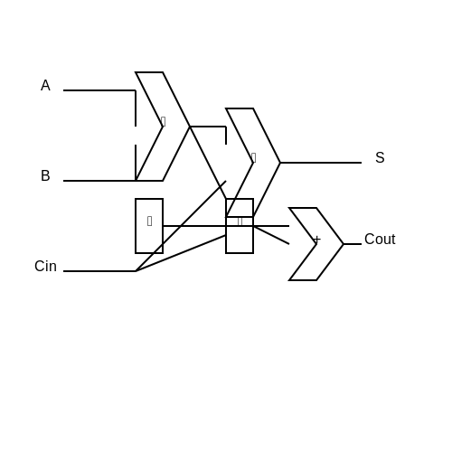
Arithmetic operations in digital systems are executed using binary adders, multipliers, and shift registers. A full adder, for instance, combines two bits and a carry-in to produce a sum and carry-out. The truth table for a full adder is derived from binary addition rules:
where S is the sum, Cout is the carry-out, and A, B, and Cin are input bits. Cascading full adders constructs multi-bit ripple-carry adders, though modern systems employ faster architectures like carry-lookahead adders to reduce propagation delay.
Hexadecimal and Memory Addressing
While binary is native to hardware, hexadecimal (base-16) simplifies human interaction with digital systems. Memory addresses, for example, are often represented in hex due to compactness. A 32-bit address spans 0x00000000 to 0xFFFFFFFF, where each hex digit corresponds to 4 binary bits. This convention is pervasive in debugging tools, assembly languages, and firmware development.
Signed Number Representations
Negative numbers in digital systems are encoded using signed-magnitude, one’s complement, or two’s complement. The latter dominates due to its arithmetic consistency and hardware efficiency. In two’s complement, the most significant bit (MSB) signifies the sign, and the value is computed as:
where n is the bit width. This representation eliminates the need for separate subtraction circuits, as A − B = A + (−B), where −B is the two’s complement of B.
Error Detection and Correction
Number systems enable error-detection codes like parity bits and cyclic redundancy checks (CRC). Parity adds a single bit to ensure an even (or odd) count of 1s, detecting single-bit errors. CRC, however, uses polynomial division over binary fields to detect burst errors in data transmission. For example, a CRC-8 generator polynomial might be:
More advanced codes, such as Hamming codes, correct errors by embedding redundant bits at power-of-two positions, enabling single-error correction and double-error detection.
Digital Signal Processing (DSP)
Fixed-point and floating-point representations are critical in DSP. Fixed-point uses integer arithmetic with implicit scaling, while floating-point adheres to standards like IEEE 754, which structures a number as:
where s is the sign bit, m the mantissa, and e the exponent. This format balances dynamic range and precision, essential for algorithms like Fast Fourier Transforms (FFT).
Case Study: Binary-Coded Decimal (BCD)
BCD encodes each decimal digit as a 4-bit binary sequence, avoiding rounding errors in financial systems. For instance, the decimal number 59 is represented as 0101 1001. Though less storage-efficient than pure binary, BCD simplifies decimal arithmetic and display interfacing, as seen in seven-segment decoders.
2. Basics of the Decimal System
2.1 Basics of the Decimal System
The decimal system, also known as the base-10 numbering system, is the most widely used numeral system in modern computation and engineering. Its foundation lies in the use of ten distinct digits (0 through 9), where each position represents a power of 10. The system's ubiquity stems from its alignment with human anatomy—specifically, the ten fingers—making it an intuitive choice for early civilizations.
Positional Notation and Weighted Values
In the decimal system, the value of a digit depends on its position within the number. For a general n-digit decimal number D represented as dn-1dn-2...d0, its numerical value is given by:
For example, the number 4375 decomposes as:
Fractional Representation
The decimal system extends to fractional values using negative powers of 10. A number F represented as d1d2...dm.d-1d-2...d-k has the value:
For instance, 82.614 resolves to:
Historical Context and Engineering Relevance
The decimal system's adoption was formalized by Indian mathematicians around the 5th century, later popularized in Europe through Arabic texts. Its engineering significance lies in its compatibility with SI units, where prefixes (kilo-, milli-, etc.) are strictly base-10. Digital systems often convert between binary and decimal for human-readable outputs, requiring efficient algorithms like BCD (Binary-Coded Decimal) in financial and metrological applications.
Limitations and Alternatives
While dominant, the decimal system is not universally optimal. Binary and hexadecimal systems outperform it in digital logic due to their alignment with transistor-based computation. However, decimal remains indispensable in contexts requiring exact fractional representation, such as currency handling—where floating-point binary approximations introduce rounding errors.
Positional Notation and Place Values
Positional notation is the foundation of modern numeral systems, where the value of a digit depends on its position within the number. Unlike additive systems like Roman numerals, positional systems leverage a base (or radix) b, with each digit's weight determined by bn, where n is its position index.
Mathematical Formulation
A number N in base b with k digits can be expressed as:
where di is the digit at position i (starting from 0 at the rightmost digit). For example, the decimal number 4276 decomposes as:
Key Properties
- Base determines digit range: Digits in base b range from 0 to b-1 (e.g., binary: 0-1, hexadecimal: 0-F).
- Place values grow exponentially: Each position leftward increases the weight by a factor of b.
- Zero as placeholder: Critical for distinguishing magnitudes (e.g., 101 vs. 1001 in binary).
Applications in Computing
Positional notation enables efficient hardware implementations:
- Binary circuits: ALUs use positional weights for arithmetic operations.
- Floating-point representation: IEEE 754 combines positional mantissa and exponent.
- Error detection: Checksums rely on modulo operations using place values.
Historical Context
The concept emerged independently in Babylonian (base-60) and Mayan (base-20) systems, but modern implementations trace to Indian mathematicians (5th century CE) who formalized base-10 with zero. This was later transmitted to Europe via Arabic scholars, revolutionizing computational efficiency.
Generalized Weighted Systems
Some systems use non-constant bases, such as:
where wi are position-dependent weights (e.g., factorial number system). These appear in specialized applications like permutation encoding.
2.3 Arithmetic Operations in Decimal
Addition and Subtraction
Decimal arithmetic follows the base-10 positional system, where each digit represents a power of 10. Addition and subtraction operations rely on carrying and borrowing mechanisms when sums or differences exceed 9. For example, adding 487 and 356:
Breaking it down:
- Units place: \(7 + 6 = 13\), write 3, carry 1 to the tens place.
- Tens place: \(8 + 5 + 1 = 14\), write 4, carry 1 to the hundreds place.
- Hundreds place: \(4 + 3 + 1 = 8\), yielding a final result of 843.
Multiplication
Decimal multiplication involves partial products, where each digit of the multiplier is applied to the multiplicand, shifted according to its positional weight. For instance, \(23 \times 45\):
Calculating each term:
- \(20 \times 40 = 800\)
- \(20 \times 5 = 100\)
- \(3 \times 40 = 120\)
- \(3 \times 5 = 15\)
Summing these partial products: \(800 + 100 + 120 + 15 = 1035\).
Division
Division in decimal is an iterative process of estimation, multiplication, and subtraction. Consider dividing 126 by 3:
Breaking it down:
- \(3 \times 40 = 120\) (first partial quotient).
- Subtract: \(126 - 120 = 6\).
- \(3 \times 2 = 6\) (second partial quotient).
- Final result: \(40 + 2 = 42\).
Floating-Point Arithmetic
For non-integer decimals, floating-point representation is used, adhering to IEEE 754 standards. Operations must account for precision and rounding errors. For example, adding 0.1 and 0.2:
This discrepancy arises from binary floating-point representation limitations, a critical consideration in numerical computing and high-precision engineering applications.
Real-World Applications
Decimal arithmetic underpins financial calculations, scientific measurements, and digital signal processing. In physics, floating-point precision affects simulations of quantum systems or orbital mechanics, where cumulative errors can diverge results significantly.
3. Fundamentals of Binary Numbers
3.1 Fundamentals of Binary Numbers
The binary number system is the foundation of digital electronics and computing, representing information using only two symbols: 0 and 1. Unlike the decimal system, which relies on powers of 10, binary operates on powers of 2, making it inherently compatible with the on/off states of transistors in modern integrated circuits.
Binary Representation and Place Values
In binary, each digit (or bit) represents an increasing power of 2, starting from the rightmost digit (least significant bit, LSB). The value of an n-bit binary number is computed as:
where bk is the k-th bit (0 or 1). For example, the 4-bit binary number 1101 translates to:
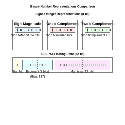
Signed Binary Representations
Negative numbers in binary are represented using three primary methods:
- Sign-Magnitude: The leftmost bit indicates the sign (0 for positive, 1 for negative), while the remaining bits represent magnitude. For example, 0101 is +5, and 1101 is -5.
- One’s Complement: Negative numbers are formed by inverting all bits of the positive counterpart. For example, -5 in 4-bit one’s complement is 1010.
- Two’s Complement: The most widely used method, where negative numbers are derived by inverting bits and adding 1. For example, -5 in 4-bit two’s complement is 1011.
Binary Arithmetic
Binary arithmetic follows analogous rules to decimal arithmetic but with a restricted digit set. Key operations include:
Addition
Binary addition proceeds bitwise from LSB to MSB, with carry propagation. For example:
Subtraction via Two’s Complement
Subtraction A − B is performed by adding A to the two’s complement of B. For example, 7 − 5 (0111 − 0101) becomes:
The overflow bit is discarded, yielding 0010 (210).
Applications in Digital Systems
Binary numbers are ubiquitous in:
- Memory Addressing: Each memory location is uniquely identified by a binary address.
- Boolean Algebra: Logical gates (AND, OR, NOT) operate on binary inputs to implement digital circuits.
- Data Encoding: Text (ASCII, Unicode), images (pixel bitmaps), and instructions (machine code) are encoded in binary.
Floating-Point Binary Representation
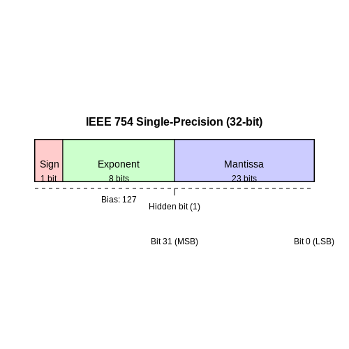
Real numbers are approximated using floating-point formats (e.g., IEEE 754), which divide a binary word into:
where s is the sign bit, m is the mantissa, and e is the exponent. For a 32-bit float, the layout is:
This representation balances range and precision, critical for scientific computing and signal processing.
3.2 Binary Arithmetic
Binary arithmetic forms the foundation of digital computation, enabling operations such as addition, subtraction, multiplication, and division using only two digits: 0 and 1. These operations are implemented in hardware via logic gates, making them essential for processors, ALUs, and embedded systems.
Binary Addition
Binary addition follows the same principles as decimal addition but with a simpler set of rules due to the base-2 system. The four possible cases for single-bit addition are:
For multi-bit numbers, addition proceeds from the least significant bit (LSB) to the most significant bit (MSB), with carries propagated leftward. Consider the addition of two 4-bit binary numbers, \( A = 1011 \) (11 in decimal) and \( B = 0110 \) (6 in decimal):
The result is \( 10001 \) (17 in decimal), with a final carry-out of 1 if the operands exceed the bit-width.
Binary Subtraction
Subtraction in binary can be performed directly or via two's complement representation, which simplifies hardware implementation. The direct method follows these rules:
For example, subtracting \( B = 0101 \) (5) from \( A = 1010 \) (10):
Two's complement subtraction involves negating the subtrahend and adding:
Binary Multiplication
Binary multiplication reduces to a series of shifts and additions, analogous to the long multiplication method in decimal. The algorithm is:
- Initialize the result to zero.
- For each bit in the multiplier, shift the multiplicand left by the bit position and add to the result if the multiplier bit is 1.
Example: Multiply \( A = 101 \) (5) by \( B = 110 \) (6):
Binary Division
Binary division uses a restoring or non-restoring algorithm, similar to long division in decimal. The steps are:
- Align the divisor with the most significant bits of the dividend.
- Subtract the divisor from the dividend; if the result is non-negative, set the quotient bit to 1 and update the dividend.
- Shift the divisor right and repeat until all bits are processed.
Example: Divide \( 1101 \) (13) by \( 101 \) (5):
The quotient is \( 10 \) (2) with a remainder of \( 11 \) (3).
Overflow and Carry Conditions
In fixed-width arithmetic, overflow occurs when the result exceeds the representable range. For unsigned numbers, a carry-out from the MSB indicates overflow. For signed numbers (two's complement), overflow is detected when the carry-in and carry-out of the MSB differ.
This condition is critical in digital signal processing (DSP) and high-performance computing, where numerical accuracy must be preserved.
Applications in Digital Systems
Binary arithmetic is implemented in hardware using combinational logic circuits. Adders, such as ripple-carry and carry-lookahead, optimize speed and power consumption. Multipliers leverage parallel architectures like Wallace trees for efficiency. These principles underpin CPUs, FPGAs, and cryptographic accelerators.
3.3 Conversion Between Binary and Decimal
Binary and decimal number systems are foundational in digital electronics, computing, and signal processing. Converting between them efficiently is essential for hardware design, algorithm optimization, and numerical analysis. Two primary methods exist: positional expansion (for binary-to-decimal) and division-by-2 (for decimal-to-binary).
Binary to Decimal Conversion
Each bit in a binary number represents a power of 2, weighted by its position. The decimal equivalent is the sum of each bit multiplied by \(2^n\), where \(n\) is its zero-indexed position from the right. For an \(m\)-bit binary number \(B = b_{m-1}b_{m-2}...b_0\):
For example, converting \(1011_2\) to decimal:
Decimal to Binary Conversion
To convert a decimal number \(D\) to binary, repeatedly divide \(D\) by 2 and record the remainders. The binary representation is the sequence of remainders read in reverse order. For \(D = 11_{10}\):
- \(11 \div 2 = 5\) (remainder 1)
- \(5 \div 2 = 2\) (remainder 1)
- \(2 \div 2 = 1\) (remainder 0)
- \(1 \div 2 = 0\) (remainder 1)
Reading the remainders from last to first yields \(1011_2\).
Fractional Conversions
For fractional parts, multiply the decimal fraction by 2 and extract the integer part iteratively. For \(0.375_{10}\):
- \(0.375 \times 2 = 0.75\) → 0
- \(0.75 \times 2 = 1.5\) → 1
- \(0.5 \times 2 = 1.0\) → 1
The fractional binary representation is \(0.011_2\).
Practical Considerations
In hardware, binary-decimal conversion is often handled by dedicated algorithms or lookup tables to optimize speed. Floating-point numbers use standardized formats (IEEE 754) where conversion requires handling exponents and mantissas separately.
Here, \(s\) is the sign bit, \(m\) is the mantissa, and \(e\) is the exponent.
4. Octal Number System: Basics and Conversions
Octal Number System: Basics and Conversions
The octal number system, or base-8, is a positional numeral system that uses eight distinct symbols: 0, 1, 2, 3, 4, 5, 6, and 7. Each position in an octal number represents a power of 8, with the rightmost digit representing 80, the next representing 81, and so on. This system is particularly useful in computing and digital systems due to its compact representation of binary-coded values.
Octal to Decimal Conversion
To convert an octal number to its decimal equivalent, expand each digit as a power of 8 and sum the results. For example, the octal number 3458 converts to decimal as follows:
Decimal to Octal Conversion
Converting a decimal number to octal involves repeated division by 8 and recording the remainders. For instance, converting 22910 to octal:
Reading the remainders from bottom to top gives the octal equivalent: 3458.
Octal to Binary Conversion
Each octal digit maps directly to a 3-bit binary sequence, making conversions straightforward. The table below shows the binary equivalents of octal digits:
| Octal Digit | Binary Equivalent |
|---|---|
| 0 | 000 |
| 1 | 001 |
| 2 | 010 |
| 3 | 011 |
| 4 | 100 |
| 5 | 101 |
| 6 | 110 |
| 7 | 111 |
For example, 3458 converts to binary as:
Binary to Octal Conversion
To convert binary to octal, group the binary digits into sets of three (starting from the right) and replace each group with its corresponding octal digit. For example, the binary number 0111001012 converts as:
Applications of the Octal System
The octal system was historically significant in early computing systems, particularly those with word lengths divisible by three (e.g., 12-bit, 24-bit architectures). Modern applications include Unix file permission notation, where three octal digits represent read, write, and execute permissions for user, group, and others.
In digital logic design, octal provides a more compact representation of binary states, simplifying the interpretation of memory dumps and register values. Its use has diminished with the prevalence of hexadecimal (base-16), but it remains relevant in specific legacy systems and educational contexts.
4.2 Hexadecimal Number System: Basics and Conversions
Fundamentals of Hexadecimal Representation
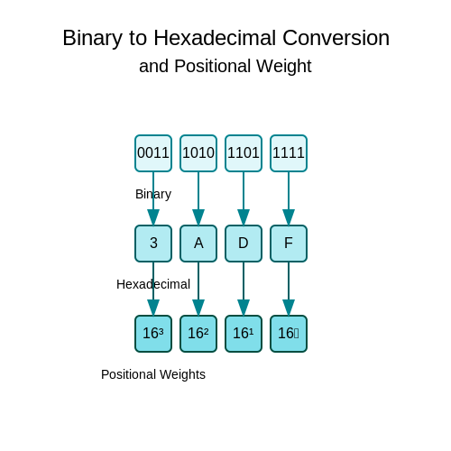
The hexadecimal (base-16) number system extends the compactness of binary and octal representations by utilizing sixteen distinct symbols: 0–9 followed by A–F, where A = 10, B = 11, ..., F = 15. Its primary advantage lies in its direct mapping to binary—each hexadecimal digit corresponds to exactly four binary digits (bits), simplifying the representation of large binary numbers. This property is exploited in memory addressing, digital signal processing, and computer graphics, where compactness and binary compatibility are critical.
Positional Notation and Weighted Expansion
A hexadecimal number H with digits dndn-1...d0 expands to its decimal equivalent via the weighted sum:
For example, the hexadecimal value 1A3F converts to decimal as:
Binary-Hexadecimal Conversion
The bidirectional conversion between binary and hexadecimal is streamlined by grouping bits into sets of four, starting from the least significant bit (LSB). Padding with leading zeros ensures complete groups. For instance, the binary number 1101011011 is segmented as 0011 0101 1011, translating to 35B in hexadecimal.
Decimal-to-Hexadecimal Conversion
To convert a decimal number to hexadecimal, iterative division by 16 collects remainders, which map to hexadecimal digits. For 42710:
- 427 ÷ 16 = 26, remainder 11 (B)
- 26 ÷ 16 = 1, remainder 10 (A)
- 1 ÷ 16 = 0, remainder 1 (1)
Reading remainders in reverse yields 1AB16.
Practical Applications
Hexadecimal notation is ubiquitous in:
- Memory Addressing: 32-bit or 64-bit addresses are concisely represented as 8 or 16 hex digits.
- Color Encoding: RGB values in web design (e.g., #FF5733) use hex triplets for red, green, and blue intensities.
- Debugging: Machine code and register dumps are often displayed in hex for readability.
Signed Hexadecimal and Two’s Complement
Negative values in hexadecimal follow two’s complement conventions. The range of an n-digit hex number in two’s complement is −8 × 16n−1 to 8 × 16n−1 − 1. For example, an 8-bit two’s complement hex value E7 converts to decimal by inverting bits (18) and adding 1: −1910.
4.3 Practical Uses in Computing
Number systems form the backbone of modern computing, with binary, hexadecimal, and octal representations enabling efficient data manipulation, storage, and transmission. Their applications span low-level hardware design to high-level software optimization.
Binary in Digital Logic and Hardware
Binary numbers directly map to the on/off states of transistors in digital circuits. A voltage level above a threshold represents 1, while a level below represents 0. This abstraction allows Boolean algebra to be implemented physically using logic gates. For example, the AND operation between two binary digits A and B is computed as:
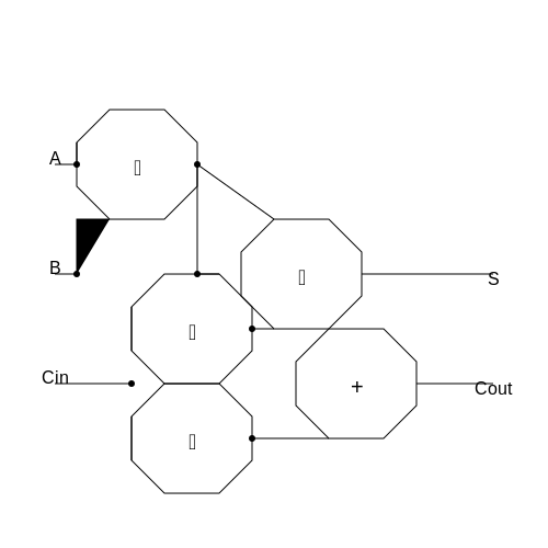
Combinational circuits built from these gates perform arithmetic operations. A full adder, for instance, sums three binary inputs (A, B, and carry-in Cin) to produce a sum (S) and carry-out (Cout):
Hexadecimal in Memory Addressing and Debugging
Hexadecimal (base-16) compactly represents binary data, with each digit corresponding to four bits. Memory addresses, such as 0xFFFF0000, are typically displayed in hex for readability. Debuggers and disassemblers use hex dumps to display raw memory contents, where a 32-bit value like 0xDEADBEEF is more interpretable than its binary equivalent 11011110101011011011111011101111.
Octal in Unix File Permissions
Unix-based systems encode file permissions using octal notation. Each digit represents a triplet of bits for read (4), write (2), and execute (1) permissions. For example, chmod 755 sets:
- 7 (111): Owner has read, write, execute
- 5 (101): Group has read, execute
- 5 (101): Others have read, execute
Floating-Point Representation
The IEEE 754 standard encodes real numbers in binary using a sign bit, exponent, and mantissa. A 32-bit float is structured as:
where S is the sign, M the 23-bit mantissa, and E the 8-bit exponent. This representation balances range and precision but introduces rounding errors, as seen in the infamous 0.1 + 0.2 ≠ 0.3 discrepancy due to binary fractions.
Error Detection and Correction
Parity bits and Hamming codes leverage binary properties to detect and correct errors. A Hamming (7,4) code appends three parity bits to four data bits, enabling single-error correction via syndrome calculation:
The syndrome s1s2s3 directly maps to the erroneous bit position.
5. Decimal to Binary, Octal, and Hexadecimal
5.1 Decimal to Binary, Octal, and Hexadecimal
Decimal to Binary Conversion
The conversion of a decimal number to binary involves repeated division by 2 and tracking the remainders. For a given decimal number N, the binary representation is obtained by concatenating the remainders in reverse order. Mathematically, this can be expressed as:
Where di ∈ {0,1}. For example, converting 2910 to binary:
- 29 ÷ 2 = 14, remainder 1 (LSB)
- 14 ÷ 2 = 7, remainder 0
- 7 ÷ 2 = 3, remainder 1
- 3 ÷ 2 = 1, remainder 1
- 1 ÷ 2 = 0, remainder 1 (MSB)
Reading the remainders from bottom to top gives 111012. This method is fundamental in digital systems where binary representation is necessary for logic operations and memory storage.
Decimal to Octal Conversion
Octal systems (base-8) are particularly useful in computing for representing binary data more compactly. The conversion process mirrors binary conversion but uses division by 8:
Where oi ∈ {0,1,...,7}. Converting 9510 to octal:
- 95 ÷ 8 = 11, remainder 7
- 11 ÷ 8 = 1, remainder 3
- 1 ÷ 8 = 0, remainder 1
The octal representation is 1378. Octal is often used in Unix file permissions and legacy assembly languages.
Decimal to Hexadecimal Conversion
Hexadecimal (base-16) is ubiquitous in computer science for memory addressing and data encoding. The conversion requires division by 16, with remainders mapped to symbols 0-9 and A-F:
For 25510:
- 255 ÷ 16 = 15, remainder 15 (F)
- 15 ÷ 16 = 0, remainder 15 (F)
Resulting in FF16. Hexadecimal simplifies binary data representation (e.g., RGB colors, MAC addresses) by grouping 4 bits per hex digit.
Fractional Decimal Conversions
For fractional numbers, multiply the fractional part by the target base repeatedly and collect integer parts. For 0.62510 to binary:
- 0.625 × 2 = 1.25 → 1 (MSB)
- 0.25 × 2 = 0.5 → 0
- 0.5 × 2 = 1.0 → 1 (LSB)
Yielding 0.1012. This method is critical in floating-point arithmetic and numerical analysis.
Practical Considerations
Signed numbers use two's complement in binary, while octal/hex rely on implicit sign handling. Precision must be considered for fractional conversions due to potential infinite representations (e.g., 0.110 = 0.0001100110011...2). Modern processors optimize these conversions via dedicated instructions (e.g., x86 FBSTP).
5.2 Binary to Octal and Hexadecimal
Binary to Octal Conversion
The conversion from binary to octal leverages the fact that octal (base-8) is a power of binary (base-2), specifically \(8 = 2^3\). This allows grouping binary digits into sets of three, starting from the least significant bit (LSB), and directly mapping each group to its corresponding octal digit. If the number of bits is not a multiple of three, leading zeros are added to complete the grouping.
This method is computationally efficient and widely used in digital systems where binary data needs to be represented compactly. For example, Unix file permissions are often displayed in octal due to their three-bit structure (read, write, execute).
Binary to Hexadecimal Conversion
Hexadecimal (base-16) is another power of binary (\(16 = 2^4\)), enabling a similar grouping technique but with four bits per group. Each 4-bit binary segment maps directly to a hexadecimal digit (0–9, A–F). Leading zeros are added if necessary to ensure complete groupings.
Hexadecimal notation is prevalent in computer engineering for memory addressing, assembly language programming, and debugging, as it concisely represents large binary values. For instance, a 32-bit memory address like 0xDEADBEEF is more readable than its binary equivalent.
Practical Applications
Microcontroller Programming: Hex files are used to flash firmware onto embedded systems, as they balance human readability with machine efficiency. Debuggers often display register values in hex to simplify interpretation.
Networking: IPv6 addresses are written in hexadecimal to reduce their length compared to binary or decimal representations. For example, 2001:0db8:85a3::8a2e:0370:7334.
Algorithmic Implementation
The following pseudocode outlines the binary-to-octal conversion process, adaptable to hexadecimal by changing the group size:
  def binary_to_octal(binary_str):
      # Pad with leading zeros to make length divisible by 3
      padding = (3 - len(binary_str) % 3
      binary_str = '0' * padding + binary_str
      octal_digits = []
      for i in range(0, len(binary_str), 3):
          chunk = binary_str[i:i+3]
          octal_digits.append(str(int(chunk, 2)))
      return ''.join(octal_digits)
5.3 Octal and Hexadecimal to Binary
Direct Conversion from Octal to Binary
Octal (base-8) and binary (base-2) systems share a direct relationship due to the power-of-two alignment (8 = 23). Each octal digit maps to a 3-bit binary sequence, making conversion straightforward. The following table summarizes the mapping:
To convert an octal number to binary, replace each digit with its corresponding 3-bit binary triplet. For example:
Hexadecimal to Binary Conversion
Hexadecimal (base-16) similarly relates to binary via 16 = 24, meaning each hex digit corresponds to a 4-bit binary sequence. The extended mapping includes alphabetic digits:
Conversion involves substituting each hex digit with its 4-bit equivalent. For instance:
Practical Applications
These conversions are foundational in:
- Computer architecture: Memory addressing and instruction encoding often use hex/octal shorthand for binary data.
- Digital logic design: FPGA configurations and microcontroller registers frequently display values in hex for readability.
- Network protocols: IPv6 addresses and MAC addresses are represented in hexadecimal to compactly encode 128-bit and 48-bit binary values.
Common Pitfalls and Edge Cases
Leading/trailing zeros must be preserved to maintain bit-width alignment. For example:
Similarly, fractional values require zero-padding after the radix point:
Algorithmic Implementation
For programmatic conversion (e.g., in Python), precomputed lookup tables optimize performance. Below is an example for hexadecimal conversion:
hex_to_bin = {
    '0': '0000', '1': '0001', '2': '0010', '3': '0011',
    '4': '0100', '5': '0101', '6': '0110', '7': '0111',
    '8': '1000', '9': '1001', 'A': '1010', 'B': '1011',
    'C': '1100', 'D': '1101', 'E': '1110', 'F': '1111'
}

def hex2binary(hex_str):
    return ''.join(hex_to_bin[digit] for digit in hex_str.upper())
6. Representation of Signed Numbers
6.1 Representation of Signed Numbers
Signed Magnitude Representation
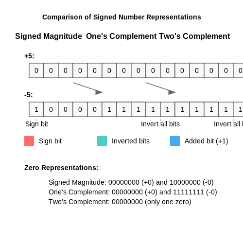
The most intuitive method for representing signed numbers is the signed magnitude approach, where the leftmost bit (most significant bit, MSB) acts as the sign bit. A 0 denotes a positive number, while a 1 denotes a negative number. The remaining bits represent the absolute value. For an n-bit number, the range is:
For example, in 8-bit signed magnitude, +5 is 00000101, and -5 is 10000101. While straightforward, this method has drawbacks: it requires separate logic for addition and subtraction, and there are two representations of zero (+0 and -0), complicating arithmetic operations.
Two's Complement Representation
The two's complement system resolves these issues and is the dominant method in modern computing. A positive number is represented normally, while its negative counterpart is obtained by inverting all bits and adding 1. The range for an n-bit two's complement number is:
For example, -5 in 8-bit two's complement is derived as follows:
This representation simplifies hardware design, as the same circuitry handles addition and subtraction. Overflow occurs when operations exceed the representable range, detectable when the carry into the sign bit differs from the carry out.
One's Complement and Offset Binary
One's complement represents negative numbers by inverting all bits of the positive counterpart. While simpler conceptually, it suffers from the same dual-zero problem as signed magnitude. The range is:
Offset binary (or excess-K) shifts the representation by a bias (typically 2n-1), making all numbers positive. This is useful in analog-to-digital converters and floating-point exponents. The value is calculated as:
Practical Applications
Two's complement is ubiquitous in digital systems, from microprocessors to FPGAs, due to its arithmetic efficiency. Signed magnitude persists in floating-point standards (IEEE 754) for the sign bit, while offset binary appears in signal processing systems where unipolar ADCs encode bipolar signals.
Arithmetic Operations
Two's complement addition proceeds as unsigned binary addition, with overflow handled by ignoring the carry beyond the MSB. Subtraction is implemented as addition of the two's complement negative. For example:
Multiplication and division require careful handling of sign bits, often using Booth's algorithm for efficiency in hardware.
6.2 Two's Complement Notation
Two's complement is the dominant method for representing signed integers in binary systems due to its computational efficiency and elimination of redundancy present in other signed number representations. Unlike sign-magnitude or one's complement, two's complement ensures a single representation for zero and simplifies arithmetic operations.
Mathematical Foundation
For an n-bit binary number, the two's complement representation of a negative number -x is derived by:
This equation holds for x > 0, where 2n serves as the modulus. For example, in an 8-bit system (n = 8), the representation of -5 is:
In binary, 251 translates to 11111011, which is the two's complement of 00000101 (5).
Conversion Procedure
To manually compute the two's complement of a negative number:
- Step 1: Write the positive counterpart in binary (e.g., 5 → 00000101).
- Step 2: Invert all bits (one's complement: 11111010).
- Step 3: Add 1 to the result (11111010 + 1 = 11111011).
This method avoids direct subtraction and leverages bitwise operations, making it hardware-friendly.
Arithmetic Advantages
Two's complement enables unified addition and subtraction circuits. For example, subtracting B from A is equivalent to adding A to the two's complement of B:
Overflow is naturally handled by discarding the carry-out beyond the n-th bit. Consider 8-bit addition of 127 + 1:
This yields -128, correctly wrapping around modulo 256.
Range and Overflow
An n-bit two's complement system covers:
For 8 bits, this spans -128 to 127. Overflow occurs when operations exceed this range, detectable via carry-in and carry-out mismatch of the most significant bit (MSB).
Hardware Implementation
Modern ALUs use two's complement for:
- Adders: Shared for signed and unsigned operations.
- Multipliers: Baugh-Wooley algorithm extends to signed numbers.
- Comparators: MSB indicates sign, simplifying magnitude checks.
This universality reduces transistor count and improves clock speeds in CPUs and DSPs.
Historical Context
Two's complement was first implemented in the 1949 EDSAC computer. Its adoption accelerated with the rise of integrated circuits, as it minimized logic gates for arithmetic units compared to sign-magnitude.
Practical Applications
Beyond general-purpose computing, two's complement is critical in:
- Digital Signal Processing: Efficient signed arithmetic in FFTs and filters.
- Cryptography: Enables fast modular arithmetic in RSA and ECC.
- FPGA Design: Simplifies fixed-point arithmetic pipelines.
6.3 Arithmetic with Signed Numbers
Representation of Signed Numbers
Signed numbers in binary are typically represented using one of three methods: sign-magnitude, one's complement, or two's complement. The two's complement representation is the most widely used in modern computing due to its efficient handling of arithmetic operations and elimination of the negative zero problem.
In two's complement, the most significant bit (MSB) acts as the sign bit. A 0 denotes a positive number, while a 1 denotes a negative number. To convert a positive number to its negative counterpart:
where \(\overline{N}\) is the bitwise complement of \(N\).
Addition of Signed Numbers
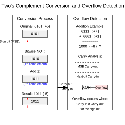
Addition in two's complement follows the same rules as unsigned binary addition. However, overflow must be considered when the result exceeds the representable range for the given bit width. Overflow occurs if:
For example, adding two 4-bit numbers \(0111 (+7)\) and \(0001 (+1)\) yields \(1000 (-8)\), which is incorrect due to overflow.
Subtraction of Signed Numbers
Subtraction is performed by adding the two's complement of the subtrahend to the minuend. This eliminates the need for a separate subtraction circuit. For example, to compute \(5 - 3\) in 4-bit two's complement:
where \(1101\) is the two's complement representation of \(-3\). The result \(0010\) is \(+2\), as expected.
Multiplication of Signed Numbers
Multiplication of signed numbers can be implemented using Booth's algorithm, which reduces the number of partial products and efficiently handles negative numbers. The algorithm examines pairs of bits in the multiplier to determine whether to add, subtract, or shift the multiplicand.
where \(A\) and \(B\) are two's complement numbers. The algorithm proceeds as follows:
- Initialize the product register with the multiplicand and extended sign bits.
- For each bit pair in the multiplier, apply Booth's rules:
- 00 or 11: Shift right.
- 01: Add multiplicand, then shift right.
- 10: Subtract multiplicand, then shift right.
Division of Signed Numbers
Division of signed numbers is typically performed using a restoring or non-restoring division algorithm. The non-restoring method is more efficient as it avoids the need to restore intermediate results. The process involves:
where \(N\) is the dividend and \(D\) is the divisor. The algorithm proceeds by iteratively shifting and conditionally adding or subtracting the divisor from the remainder.
Overflow Detection and Handling
Overflow in signed arithmetic occurs when the result of an operation cannot be represented within the given number of bits. In hardware, overflow is detected by comparing the carry into and out of the sign bit. Software implementations often rely on flag registers or explicit checks.
For example, in a 32-bit system, adding \(2^{30}\) and \(2^{30}\) would produce \(2^{31}\), which is interpreted as a negative number in two's complement, indicating overflow.
Practical Applications
Signed arithmetic is fundamental in digital signal processing (DSP), where operations on signed data are common. For instance, finite impulse response (FIR) filters require signed multiplication and accumulation. Modern processors optimize signed arithmetic using dedicated hardware units, such as multiply-accumulate (MAC) circuits.
In embedded systems, efficient signed arithmetic is critical for real-time control algorithms, where minimizing latency and power consumption is essential.
7. IEEE 754 Floating-Point Standard
7.1 IEEE 754 Floating-Point Standard
The IEEE 754 standard defines the representation and manipulation of floating-point numbers in digital systems, ensuring consistency across hardware and software implementations. It specifies binary and decimal formats, though binary formats are most prevalent in modern computing.
Basic Structure
A floating-point number under IEEE 754 is represented in three parts:
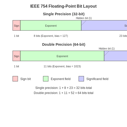
- Sign bit (1 bit): Determines whether the number is positive (0) or negative (1).
- Exponent (8 bits for single-precision, 11 bits for double-precision): A biased integer representing the power of two by which the significand is multiplied.
- Significand (23 bits for single-precision, 52 bits for double-precision): Also called the mantissa, this represents the fractional part of the number, normalized to a leading implicit bit (hidden bit).
Normalized Representation
For a normalized floating-point number, the value V is computed as:
Where:
- S is the sign bit (0 or 1).
- M is the significand (fractional part).
- E is the exponent (with bias B).
- B is the bias (127 for single-precision, 1023 for double-precision).
Special Cases
IEEE 754 defines special representations for:
- Zero: Exponent and significand both zero. Can be +0 or -0.
- Denormalized numbers: When exponent is zero but significand is non-zero, allowing gradual underflow.
- Infinity: Exponent all ones, significand zero. Can be +∞ or -∞.
- NaN (Not a Number): Exponent all ones, significand non-zero. Used for undefined operations (e.g., √-1).
Single-Precision vs. Double-Precision
| Feature | Single-Precision (32-bit) | Double-Precision (64-bit) |
|---|---|---|
| Sign Bits | 1 | 1 |
| Exponent Bits | 8 (Bias = 127) | 11 (Bias = 1023) |
| Significand Bits | 23 | 52 |
| Approx. Decimal Range | ±1.18×10-38 to ±3.4×1038 | ±2.23×10-308 to ±1.80×10308 |
Rounding Modes
IEEE 754 defines five rounding modes:
- Round to Nearest, Ties to Even (Default): Rounds to the closest representable value; if equidistant, rounds to the nearest even significand.
- Round Toward Zero: Truncation, discarding excess bits.
- Round Toward +∞: Always rounds up.
- Round Toward -∞: Always rounds down.
- Round to Nearest, Ties Away from Zero: Less common, rounds halfway cases away from zero.
Floating-Point Arithmetic
Operations follow strict rules to maintain precision and handle edge cases:
- Addition/Subtraction: Align exponents, perform operation, then normalize.
- Multiplication: Multiply significands, add exponents, adjust bias, normalize.
- Division: Divide significands, subtract exponents, adjust bias, normalize.
Practical Implications
The IEEE 754 standard is critical in scientific computing, embedded systems, and GPU architectures, where numerical consistency and precision are paramount. However, floating-point arithmetic introduces challenges:
- Loss of Precision: Some decimal numbers (e.g., 0.1) cannot be represented exactly in binary floating-point.
- Catastrophic Cancellation: Subtraction of nearly equal numbers can lead to significant relative error.
- Overflow/Underflow: Exceeding exponent limits results in ±∞ or subnormal numbers.
Example: Single-Precision Encoding
Consider the number -118.625:
- Sign bit: 1 (negative).
- Binary representation: 1110110.101 (118.625 in binary).
- Normalize: 1.110110101 × 26.
- Exponent: 6 + 127 (bias) = 133 → 10000101.
- Significand: 11011010100000000000000 (23 bits).
The final 32-bit representation is:
7.2 Single and Double Precision Formats
Floating-point representation in computing adheres to the IEEE 754 standard, which defines two primary precision formats: single (32-bit) and double (64-bit). These formats balance storage efficiency with numerical accuracy, making them indispensable in scientific computing, signal processing, and numerical simulations.
Single Precision (32-bit) Format
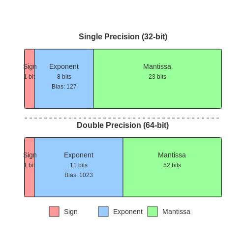
The single-precision format allocates 32 bits as follows:
- Sign bit (1 bit): Determines the number's sign (0 for positive, 1 for negative).
- Exponent (8 bits): Stored in biased form (excess-127), enabling representation of exponents from -126 to +127.
- Mantissa (23 bits): The fractional part of the significand, with an implicit leading 1 (normalized form).
The value of a single-precision number is computed as:
where S is the sign bit, M is the mantissa, and E is the exponent. Special cases include:
- E = 0, M = 0: Zero (signed).
- E = 255, M = 0: Infinity (±∞).
- E = 255, M ≠ 0: Not-a-Number (NaN).
Double Precision (64-bit) Format
Double precision extends the dynamic range and precision with 64 bits:
- Sign bit (1 bit): Same as single precision.
- Exponent (11 bits): Uses excess-1023 bias, covering exponents from -1022 to +1023.
- Mantissa (52 bits): Higher precision due to increased fractional bits.
Double precision's larger exponent and mantissa reduce rounding errors, making it essential for applications like finite element analysis and high-fidelity simulations.
Precision and Rounding Errors
Rounding errors arise from finite mantissa bits. Single precision offers ~7 decimal digits of precision, while double precision provides ~16. The relative error for a single-precision number is bounded by:
For double precision:
Practical Considerations
In hardware, single precision requires less memory bandwidth and computational resources, favoring real-time systems (e.g., GPU shaders). Double precision is preferred for iterative algorithms (e.g., numerical integration) where error accumulation must be minimized. Modern processors often include fused multiply-add (FMA) units to mitigate precision loss in chained operations.
7.3 Floating-Point Arithmetic
Floating-point arithmetic is a computational method for representing and manipulating real numbers in digital systems. Unlike fixed-point representations, floating-point numbers allow a wide dynamic range by separating the number into three components: the sign, exponent, and mantissa (or significand). The IEEE 754 standard defines the most widely used formats, including single-precision (32-bit) and double-precision (64-bit) floating-point representations.
IEEE 754 Floating-Point Representation
A floating-point number N is expressed as:
where:
- S is the sign bit (0 for positive, 1 for negative).
- M is the mantissa, a normalized fractional value in the range [1, 2) for normal numbers.
- E is the biased exponent, stored as an unsigned integer.
- B is the exponent bias (127 for single-precision, 1023 for double-precision).
The IEEE 754 single-precision format allocates:
- 1 bit for the sign (S).
- 8 bits for the exponent (E).
- 23 bits for the mantissa (M).
Normalization and Denormal Numbers
For normal numbers, the mantissa is implicitly normalized such that the leading bit is 1 (hidden bit). The exponent range is adjusted to avoid underflow and overflow:
Denormal (subnormal) numbers relax this condition when the exponent is zero, allowing representation of extremely small values at the cost of precision:
Rounding and Error Analysis
Floating-point operations introduce rounding errors due to finite precision. IEEE 754 defines several rounding modes:
- Round to Nearest (Ties to Even) – Default mode, minimizes average error.
- Round Toward Zero – Truncation.
- Round Toward +∞ / -∞ – Directed rounding for interval arithmetic.
The relative error in representing a real number x is bounded by machine epsilon (ε):
where ε is 2-23 (≈1.19×10⁻⁷) for single-precision and 2-52 (≈2.22×10⁻¹⁶) for double-precision.
Floating-Point Arithmetic Operations
Basic operations (addition, subtraction, multiplication, division) follow these steps:
- Alignment – Adjust exponents to match the larger operand.
- Computation – Perform the operation on the mantissas.
- Normalization – Shift the result to restore the leading 1.
- Rounding – Apply the selected rounding mode.
Multiplication and division are simpler since exponent addition/subtraction is independent of mantissa operations:
Special Cases and Exceptions
IEEE 754 defines special floating-point values:
- Zero – Signed zeroes (±0) to preserve sign in underflow.
- Infinity (±∞) – Result of overflow or division by zero.
- NaN (Not a Number) – Result of invalid operations (e.g., √-1, 0/0).
Exceptions (e.g., overflow, underflow, division by zero) trigger flags that can be checked for error handling.
Practical Considerations in Scientific Computing
Floating-point arithmetic is ubiquitous in numerical simulations, but precision loss must be managed:
- Catastrophic cancellation – Subtraction of nearly equal numbers amplifies relative error.
- Accumulated rounding errors – Long sequences of operations require stable algorithms (e.g., compensated summation).
- Condition number – Measures sensitivity to input perturbations; ill-conditioned problems exacerbate floating-point errors.
High-performance computing often employs fused multiply-add (FMA) operations, which compute a×b + c with a single rounding step, improving accuracy and speed.
8. Recommended Books and Papers
8.1 Recommended Books and Papers
- PDF Computer Arithmetic: Principles, Architectures, and VLSI Design - ETH Z — 3 Number Representations 10 3.1 Binary Number Systems (BNS) 10 3.2 Gray Numbers 13 3.3 Redundant Number Systems 14 3.4 Residue Number Systems (RNS) 16 3.5 Floating-Point Numbers 18 3.6 Logarithmic Number System 19 3.7 Antitetrational Number System 19 3.8 Composite Arithmetic 20 3.9 Round-Off Schemes 21 4 Addition 22 4.1 Overview 22 4.2 1-Bit ...
- PDF FOUNDATIONS OF DIGITAL ELECTRONICS - University of Nairobi — 1: Number Systems and Codes 1 1.1 The binary number system 1 1.2 Unsigned binary arithmetic 5 1.3 Signed binary arithmetic 7 1.4 The octal number system 13 1.5 The hexadecimal number system 16 1.6 Number codes 20 1.7 Character codes 27 1.8 Floating point numbers 29 1.9 Problems 34 2: Basic Combinational Logic Circuits 35 2.1 Elements of Boolean ...
- INTRODUCTION TO DIGITAL SYSTEMS - Wiley Online Library — 1.10 Future of Digital Systems 7 Problems 8 2 Number Systems 9 2.1 Objectives 9 2.2 Bases and Number Systems 9 2.3 Number Conversions 11 2.4 Data Organization 13 2.5 Signed and Unsigned Numbers 13 2.6 Binary Arithmetic 16 2.7 Addition of Signed Numbers 17 2.8 Binary-Coded Decimal Representation 19 2.9 BCD Addition 20 Problems 21 3 Boolean ...
- PDF Introduction to Digital Electronics - Agner — 1. Number systems 1.1. Decimal, binary, and hexadecimal numbers We all know the decimal number system. For example, 2019 means 2*1000 + 0*100 + 1*10 + 9*1. The numbers 2, 0, 1, 9 are called the digits of the number 2019. If we want to describe this mathematically, we will call the rightmost digit d 0, the next digit d 1, etc. If there are n ...
- PDF Number Systems - Wiley — Number Systems Thestudyof ... Similarly, voltage across a certain component in an electronic circuit may be measured as 6.5 V or 6.49 V or 6.487 V or 6.4869 V. The underlying concept in this ... different digits in the octal number system are 80,81,82 and so on (for the integer part) and 8−1,8−2, 8−3 and so on ...
- Chapter 8: Number Systems Used in Digital Electronics — 8.1 OVERVIEW. There are four systems of arithmetic which are often used in digital circuits. These systems are: Decimal: The decimal system has a base (or radix) of 10. Therefore it uses ten different symbols to represent numbers.
- Digital Electronics 1 - Wiley Online Library — 1) Number Systems; 2) Logic Gates; 3) Function Blocks of Combinational Logic; 4) Systematic Methods for the Simplification of Logic Functions. 2. The reader This book is an indispensable tool for all engineering students in bachelors or masters course who wish to acquire detailed and practical knowledge of digital electronics.
- DIGITAL ELECTRONICS: CIRCUITS AND SYSTEMS - ResearchGate — Hexa decimal number system 26 . 2.6. ... Logic operation in electronic circuit 41 . 3.5. ... In this final chapter we reflect on the papers presented in this book. As such, the different ...
- (PDF) Number Systems - Academia.edu — Chapter 5 may seem to be a digression from the main thrust of the book: we introduce primes and factorisations, representations of numbers in any base (we avoid giving base ten its usual pre-eminence), and modular arithmetic, which will all reappear later in the book; but the only new number systems defined in this chapter are the finite rings ...
- PDF 01. Number Systems - madeeasypublications.org — or transmitted in any form or by any means (electronic, mechanical, photo-copying, recording or otherwise), without the prior written permission of the above mentioned publisher of this book. MADE EASY Publications Pvt. Ltd. has taken due care in collecting the data and providing the solutions, before publishing this book.
8.2 Online Resources and Tutorials
- Number Systems | Electronics Tutorial — Number Systems in Digital Electronics Number system basically divided into following broad categories. To learn about basic of base values of commonly used number systems. Decimal Binary. Octal. Hexadecimal. Binary Number System Binary Numbers Binary-to-Decimal Conversion Decimal Number System Decimal-to-Binary Conversion Decimal-to-Hexadecimal Conversion Decimal-to-Octal Conversion ...
- Digital Electronics - Number Systems - Online Tutorials Library — Digital number systems form the foundation of the modern computing technologies and digital electronics. They are used to represent, process, and manipulate the information using a digital system.
- Math 8 - 8.NS.2 Real Numbers System - Google Sites — Number and Number Sense 8.NS.2 Subsets of the Real Number System
- PDF Introduction to Digital Electronics - Agner — 1.1. Decimal, binary, and hexadecimal numbers We all know the decimal number system. For example, 2019 means 2*1000 + 0*100 + 1*10 + 9*1. The numbers 2, 0, 1, 9 are called the digits of the number 2019.
- Number Systems in Digital Electronics — • Electronic systems may use a variety of different number systems, (e.g. Decimal, Hexadecimal, Octal, Binary). • The number system in use can be identified by its radix (10, 16, 8, 2).
- SOL 8.2 Real Number System Flashcards | Quizlet — Study with Quizlet and memorize flashcards containing terms like counting number, natural number, irrational number and more.
- Chapter 8: Number Systems Used in Digital Electronics | GlobalSpec — The binary system is extensively used by digital systems like digital computers which operate on binary information. The octal system has certain advantages in digital work because it requires less circuitry to get information into and out of a digital system.
- PDF Lecture Notes for Digital Electronics - University of Oregon — The number of bits of memory (e.g. of flip-flops) required to specify the m states is at minimum n = log2(m). Make a state diagram which shows all states, inputs, and outputs.
- SOL 8.2 Real Number System - YouTube — No description has been added to this video....more
- 8.2 Real Number System Vocabulary Review - Desmos — by Mary Harris
8.3 Advanced Topics in Number Systems
- PDF AN 83: Binary Numbering Systems - Intel — Table 1 summarizes the binary numbering systems described in this application note. For each numbering system, the number range is provided for an N-bit number. For fractional numbering systems, the number range is provided for an N + M-bit number, where N is the integer part of the number and M is the fractional part of the number.
- INTRODUCTION TO DIGITAL SYSTEMS - Wiley Online Library — 1.10 Future of Digital Systems 7 Problems 8 2 Number Systems 9 2.1 Objectives 9 2.2 Bases and Number Systems 9 2.3 Number Conversions 11 2.4 Data Organization 13 2.5 Signed and Unsigned Numbers 13 2.6 Binary Arithmetic 16 2.7 Addition of Signed Numbers 17 2.8 Binary-Coded Decimal Representation 19 2.9 BCD Addition 20 Problems 21 3 Boolean ...
- PDF FOUNDATIONS OF DIGITAL ELECTRONICS - University of Nairobi — 1: Number Systems and Codes 1 1.1 The binary number system 1 1.2 Unsigned binary arithmetic 5 1.3 Signed binary arithmetic 7 1.4 The octal number system 13 1.5 The hexadecimal number system 16 1.6 Number codes 20 1.7 Character codes 27 1.8 Floating point numbers 29 1.9 Problems 34 2: Basic Combinational Logic Circuits 35 2.1 Elements of Boolean ...
- Computer Number Systems - ACSL Category Descriptions — Different Number Systems. A number system is the way we name and represent numbers. The number system we use in our daily life is known as decimal number system or base 10 because it is based on 10 different digits: 0, 1, 2, ..., 8, and 9. The base of number is written as subscript to a number. For example, the decimal number "twelve thousand three hundred and forty-five" is written as $12345 ...
- Assignment-1: Digital Electronics: CT 304-N Semester: 3 (CE ... - Scribd — This document contains a 12 question assignment on number systems and codes for a Digital Electronics course. The questions cover converting between decimal, binary, octal, and hexadecimal number systems, computing 1's and 2's complements, subtracting numbers using complements, and representing a decimal number using various codes.
- PDF Number Systems - Wiley — Similarly, the binary number system with only two independent digits, 0 and 1, is a radix-2 number system. The octal and hexadecimal number systems have a radix (or base) of 8 and 16 respectively. We will see in the following sections that the radix of the number system also determines the other two characteristics.
- PDF Chapter 3: Number Systems - University of Wisconsin-Madison — General number system (Base-B numbers) Any number can be used as a base for a number system. • If the number is less than (or equal) to 10, we can use a subset of the digits 0-9 for the symbols. • if the base is greater than 10, we use letters as additional symbols so that each digit takes up only one place in the numeral. o Example ...
- CS301: Practice with Number Systems - Saylor Academy — The binary numeral system, or base-2 number system, represents numeric values using two symbols: 0 and 1. More specifically, the usual base-2 system is a positional notation with a radix of 2. Because of its straightforward implementation in digital electronic circuitry using logic gates, the binary system is used internally by almost all ...
- PDF Lecture Notes for Digital Electronics - University of Oregon — 2. Add some number to −2MSB to get the number you want. For 4-bit numbers an example of nding the 2's complement of 5 is −5=−8+3 = 1000+0011 = 1011. 1.2.2 Hexadecimal Representation It is very often quite useful to represent blocks of 4 bits by a single digit. Thus in base
- PDF Number System - BS Publications — 3. Implement the digital systems in terms of logic circuits. 4. Understand the concepts and techniques of code conversion. 1.1 DIGITAL ELECTRONICS Digital electronics is a branch of electronics which deals with arithmetic of digits, design of digital and logic circuits. To control and process various systems, digital circuits are mostly used.