Renewable Energy Systems
1. Definition and Importance of Renewable Energy
1.1 Definition and Importance of Renewable Energy
Fundamental Definition
Renewable energy systems harness energy from naturally replenishing sources, such as solar irradiance, wind kinetic energy, geothermal heat, and hydroelectric potential. Unlike fossil fuels, these sources exhibit near-zero depletion rates on human timescales. The defining characteristic is the sustainability condition:
where \( E \) represents the total available energy and \( E_{\text{extracted}} \) denotes human consumption. This inequality must hold true over multi-decadal periods for a source to qualify as renewable.
Energy Conversion Mechanisms
All renewable systems rely on fundamental physics principles for energy conversion:
- Photovoltaic Effect: Semiconductor bandgap excitation by photons (\( E_g \geq h\nu \))
- Electromagnetic Induction: Faraday's law (\( \mathcal{E} = -N\frac{d\Phi_B}{dt} \)) in wind turbines
- Thermodynamic Cycles: Rankine or Kalina cycles for geothermal plants
Global Energy Context
The 2023 IEA World Energy Outlook indicates renewables now constitute 29.3% of global electricity generation, with projected growth to 47% by 2030. This transition responds to three critical imperatives:
| Factor | Impact Metric | Renewable Advantage |
|---|---|---|
| Climate Change | gCO₂eq/kWh | Wind: 11, vs Coal: 820 |
| Energy Security | Import Dependency | Localized generation |
| Economic | LCOE ($/MWh) | Solar PV: 37, vs Gas: 59 |
Technical Challenges
Despite advantages, renewable integration presents unique engineering hurdles:
where \( \eta \) is conversion efficiency and \( \tau \) the storage time constant. The intermittent nature of sources like solar and wind requires sophisticated grid management through:
- Inertia emulation with power electronics
- Distributed energy resource management systems (DERMS)
- Advanced forecasting using machine learning
Material Science Considerations
Emerging technologies push material limits:
- Perovskite solar cells now achieve 33.7% efficiency (NREL 2023)
- NdFeB magnets in wind turbines require rare-earth element alternatives
- Solid-state batteries for energy storage (500+ Wh/kg theoretical)
1.2 Key Differences Between Renewable and Non-Renewable Energy
Energy Source Regeneration Timescales
The fundamental distinction lies in regeneration rates. Renewable sources like solar, wind, and hydroelectric power are replenished on human timescales, typically governed by natural cycles:
where τ represents the regeneration period. In contrast, fossil fuels exhibit geological timescales:
This difference manifests in the sustainability quotient (Qs), defined as the ratio of consumption rate to regeneration rate:
Energy Density and Infrastructure Requirements
Non-renewable sources exhibit higher volumetric energy densities, with coal at ~24 MJ/kg compared to wind's ~0.5 MJ/m3. This necessitates distinct infrastructure scaling:
- Fossil plants achieve ~1 GW output from <1 km2
- Solar farms require ~5 km2 for equivalent output
- Wind farms need ~50 km2 land area
The power density differential is quantified by:
Thermodynamic Efficiency Limits
Renewable systems operate under different thermodynamic constraints. Photovoltaic cells are fundamentally limited by the Shockley-Queisser limit:
where Jsc is short-circuit current, Voc open-circuit voltage, and FF the fill factor. This contrasts with Carnot-limited thermal plants:
Grid Integration Challenges
The intermittent nature of renewables introduces stability considerations. The capacity factor (Cf) difference is substantial:
Typical values range from 20-40% for renewables versus 70-90% for fossil/nuclear. This necessitates advanced grid management through:
- Inertia emulation with power electronics
- Predictive generation forecasting
- Distributed energy storage systems
Environmental Impact Metrics
Lifecycle analysis reveals order-of-magnitude differences in emission intensities:
| Source | CO2 (gCO2/kWh) | Land Use (m2/GWh) |
|---|---|---|
| Coal | 820-1010 | 0.2-0.4 |
| Solar PV | 18-48 | 3-10 |
| Wind | 7-16 | 2-5 |
The externality cost differential becomes significant when considering the social cost of carbon (SCC), currently estimated at $51/ton CO2.
1.3 Global Trends and Adoption Rates
Current Market Penetration and Growth Projections
The global renewable energy sector has experienced exponential growth over the past two decades, driven by declining costs, policy incentives, and technological advancements. Solar photovoltaic (PV) capacity has grown at a compound annual growth rate (CAGR) of approximately 22% since 2010, while wind energy has expanded at a CAGR of 14%. The International Energy Agency (IEA) projects that renewables will account for over 42% of global electricity generation by 2030 under current policy scenarios, with solar and wind contributing nearly 25%.
Where n is the number of years. For solar PV, if installed capacity grew from 40 GW in 2010 to 850 GW in 2022, the CAGR is calculated as:
Regional Disparities in Adoption
Adoption rates vary significantly by region due to differences in resource availability, policy frameworks, and economic conditions:
- Europe: Leads in per capita renewable energy deployment, with countries like Germany and Denmark achieving over 50% renewable electricity penetration.
- China: Dominates in absolute capacity, accounting for 40% of global solar PV and 35% of wind installations as of 2023.
- United States: Growth is uneven, with states like California and Texas driving most additions due to favorable policies and resource potential.
- Developing Nations: Face financing and infrastructure barriers but show rapid growth in distributed solar, particularly in India and sub-Saharan Africa.
Technological and Economic Drivers
The levelized cost of electricity (LCOE) for renewables has fallen dramatically, making them competitive with fossil fuels. Between 2010 and 2023:
- Solar PV LCOE dropped by 89%, from $$0.38/kWh to $$0.04/kWh.
- Onshore wind LCOE declined by 70%, from $$0.09/kWh to $$0.03/kWh.
Where It is capital expenditure, Mt is operational costs, Ft is fuel costs (zero for renewables), Et is energy output, and r is the discount rate.
Policy and Investment Trends
Global investment in renewable energy reached $$500 billion in 2022, with private sector funding surpassing public financing. Key policy mechanisms include:
- Feed-in Tariffs (FiTs): Guaranteed pricing for renewable energy producers, widely used in early adoption phases.
- Renewable Portfolio Standards (RPS): Mandates for utilities to source a percentage of power from renewables.
- Auction Systems: Competitive bidding for renewable projects, driving cost reductions.
Emerging Technologies and Future Outlook
Next-generation technologies are poised to further disrupt the energy landscape:
- Offshore Wind: Floating turbine technology expands viable locations, with costs projected to fall below $$50/MWh by 2030.
- Green Hydrogen: Electrolyzers powered by renewables could decarbonize hard-to-abate sectors like steel and shipping.
- Perovskite Solar Cells: Lab efficiencies now exceed 33%, with potential for low-cost, high-performance modules.
Global renewable capacity additions are expected to average 350 GW annually through 2030, requiring $1.3 trillion in cumulative investment to meet Paris Agreement targets.
2. Photovoltaic (PV) Technology
2.1 Photovoltaic (PV) Technology
Fundamental Principles of Photovoltaic Conversion
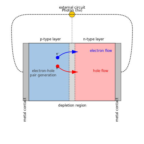
The photovoltaic effect arises from the interaction of photons with semiconductor materials, generating electron-hole pairs when photon energy exceeds the bandgap Eg. In crystalline silicon (c-Si), the most prevalent PV material, the bandgap is approximately 1.1 eV at 300 K. The maximum theoretical efficiency is constrained by the Shockley-Queisser limit, derived from detailed balance considerations:
where Jsc is the short-circuit current density, Voc the open-circuit voltage, FF the fill factor, and Pin the incident power density. For single-junction c-Si under AM1.5 spectrum, the theoretical limit is ~33%.
Device Physics and Carrier Dynamics
PV cells operate via the following sequence:
- Photon absorption creates electron-hole pairs in the depletion region or within a diffusion length of it.
- Charge separation occurs via the built-in electric field of the p-n junction.
- Carrier collection at the electrodes requires minimization of recombination losses.
The diode equation modified for illumination describes the current-voltage characteristics:
where I0 is the reverse saturation current, n the ideality factor, and IL the light-generated current.
Advanced Cell Architectures
Modern high-efficiency designs incorporate:
- Passivated emitter and rear contact (PERC): Reduces surface recombination via dielectric layers.
- Heterojunction with intrinsic thin-layer (HIT): Combines c-Si with amorphous silicon passivation.
- Tandem cells: Stacks multiple bandgap materials to better utilize the solar spectrum.
The efficiency η of a tandem cell with N junctions follows:
System-Level Considerations
Practical PV systems require:
- Maximum power point tracking (MPPT): Dynamically adjusts load impedance to operate at Pmax.
- Inverter topologies: Multilevel designs minimize harmonic distortion in grid-tied systems.
- Degradation analysis: LID (light-induced degradation) in c-Si can reduce output by 1-3% in initial exposure.
The levelized cost of energy (LCOE) for a PV plant is calculated as:
where It is investment cost, Mt maintenance cost, Et energy produced, and r the discount rate.
Emerging Technologies
Research frontiers include:
- Perovskite solar cells: Solution-processable materials with tunable bandgaps achieving >25% efficiency.
- Quantum dot PV: Enables hot-carrier extraction and multiple exciton generation.
- Thermophotovoltaics: Combines thermal emitters with low-bandgap cells for >50% theoretical efficiency.
2.2 Solar Thermal Systems
Fundamentals of Solar Thermal Energy Conversion
Solar thermal systems convert incident solar radiation into usable heat energy through absorption and thermal transfer. The efficiency of such systems depends on the absorber's ability to maximize solar irradiance capture while minimizing thermal losses. The absorbed energy Qabs is given by:
where α is the absorptivity of the surface, G is the solar irradiance (W/m²), and A is the absorber area. Conduction, convection, and radiation losses must be accounted for to determine net useful energy output.
Types of Solar Thermal Collectors
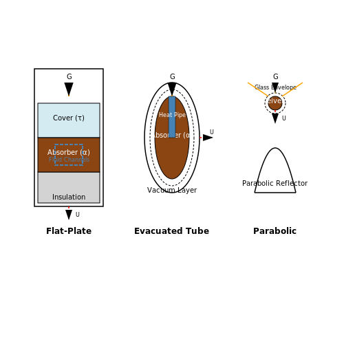
Solar thermal collectors are broadly classified into three categories based on operating temperature and design:
- Flat-Plate Collectors (FPCs): Operate at low to medium temperatures (30–80°C), consisting of an insulated metal box with a dark absorber plate and transparent cover to reduce convective losses.
- Evacuated Tube Collectors (ETCs): Utilize vacuum-sealed tubes to minimize convection and conduction losses, achieving higher efficiencies (50–70°C) than FPCs.
- Concentrating Solar Collectors (CSCs): Use mirrors or lenses to focus sunlight onto a small receiver, enabling high-temperature applications (100–400°C).
Thermodynamic Analysis of Solar Collectors
The performance of a solar collector is quantified by the thermal efficiency η, derived from the first law of thermodynamics:
where τ is the transmissivity of the cover, UL is the overall heat loss coefficient, Tabs is the absorber temperature, and Tamb is the ambient temperature.
Heat Transfer Fluids and Storage Systems
Common working fluids include water, synthetic oils, and molten salts, selected based on thermal stability and heat capacity. Thermal storage is critical for mitigating intermittency, with sensible heat storage being the most prevalent:
where m is the mass of the storage medium, cp is the specific heat capacity, and ΔT is the temperature differential.
Applications and Case Studies
Solar thermal systems are deployed in:
- Domestic Hot Water (DHW) Systems: FPCs and ETCs dominate residential applications, reducing reliance on electric or gas heating.
- Industrial Process Heat (IPH): CSCs provide steam for food processing, textile manufacturing, and chemical industries.
- Concentrated Solar Power (CSP) Plants: Parabolic troughs and solar towers generate electricity via Rankine or Brayton cycles.
Advanced Research and Emerging Technologies
Recent developments include:
- Nanofluids: Suspensions of nanoparticles in base fluids enhance thermal conductivity and absorption efficiency.
- Phase Change Materials (PCMs): Latent heat storage enables higher energy density than sensible storage.
- Hybrid PV-Thermal Systems: Simultaneously generate electricity and thermal energy, improving overall system efficiency.
2.3 Grid Integration and Storage Solutions
Challenges in Renewable Energy Grid Integration
Integrating renewable energy sources (RES) into the electrical grid introduces several technical challenges due to their intermittent nature. Unlike conventional power plants, solar and wind generation are subject to rapid fluctuations caused by weather conditions. The grid must maintain stability despite these variations, requiring advanced control strategies to balance supply and demand in real time.
The primary stability concerns include:
- Frequency regulation: RES lack inherent inertia, making frequency control more difficult during load imbalances.
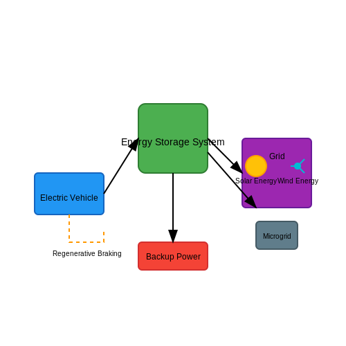
- Voltage control: Distributed generation can cause reverse power flow and voltage rise in distribution networks.
- Harmonic distortion: Power electronic converters introduce high-frequency noise that must be filtered.
Energy Storage as a Solution
Energy storage systems (ESS) mitigate intermittency by decoupling generation from consumption. The required storage capacity depends on the RES penetration level and the grid's flexibility. The key metrics for evaluating ESS include:
Where \(E_{storage}\) is the energy capacity needed to cover the deficit between generation \(P_{generation}(t)\) and demand \(P_{demand}(t)\) over time period \(t_1\) to \(t_2\).
Battery Technologies
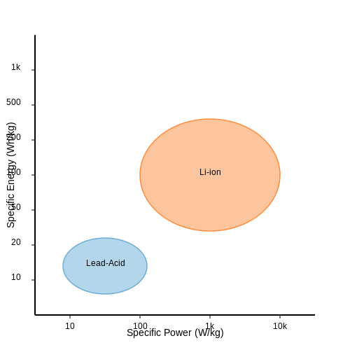
Lithium-ion batteries dominate grid-scale applications due to their high energy density (\(>200\) Wh/kg) and efficiency (\(>95\%\)). The Ragone plot below compares different battery types:
Advanced Grid Management Techniques
Modern grid integration employs several advanced technologies:
Virtual Synchronous Machines (VSM)
VSMs emulate the inertia of synchronous generators using power electronics. The control law for a VSM is:
Where \(J\) is the virtual inertia, \(\omega\) is angular frequency, \(T_m\) and \(T_e\) are mechanical and electrical torques, and \(D\) is the damping coefficient.
Model Predictive Control (MPC)
MPC optimizes grid operations by solving a finite-horizon optimization problem at each time step:
Where \(x_k\) is the state vector, \(u_k\) is the control input, and \(Q\), \(R\) are weighting matrices.
Case Study: Hornsdale Power Reserve
The 150 MW/194 MWh Tesla battery system in South Australia demonstrates successful grid integration. Key performance metrics:
- Response time: <140 ms for frequency control
- Cost savings: Reduced grid stabilization costs by AU$116 million in first two years
- Efficiency: 92% round-trip efficiency
3. Wind Turbine Mechanics and Design
3.1 Wind Turbine Mechanics and Design
Aerodynamic Principles of Wind Turbines
The mechanical energy extraction from wind relies on the aerodynamic interaction between the turbine blades and incoming airflow. The fundamental principle is governed by Bernoulli’s equation and the lift-drag mechanism of airfoil-shaped blades. The lift force, perpendicular to the relative wind direction, drives rotor rotation, while drag acts as a resistive force. The angle of attack (α) determines the efficiency of lift generation and must be optimized to prevent stall conditions.
where L is lift force, ρ is air density, v is wind velocity, CL is the lift coefficient, and A is the blade area.
Betz Limit and Maximum Power Extraction
The Betz limit defines the theoretical maximum fraction of kinetic energy that can be extracted from wind, calculated as 16/27 (≈59.3%) of the total available power. This arises from the necessity of maintaining airflow continuity downstream. The extractable power Pmax is derived from momentum theory:
Real-world turbines typically achieve 35–45% efficiency due to mechanical and electrical losses.
Blade Element Momentum (BEM) Theory
BEM theory combines momentum conservation with blade element analysis to predict turbine performance. The blade is divided into annular elements, each contributing to torque and thrust. The iterative solution balances:
- Axial induction factor (a): Reduction in wind speed due to energy extraction.
- Angular induction factor (a’): Swirl imparted to the airflow.
The local power coefficient CP for each element is:
Structural Design Considerations
Turbine blades must withstand cyclic loads from wind shear, turbulence, and gravity. Key design parameters include:
- Material selection: Carbon fiber-reinforced polymers (CFRP) for high strength-to-weight ratios.
- Taper and twist distribution: Optimized to maintain optimal angle of attack along the span.
- Fatigue resistance: Addressed through composite layup optimization and damage-tolerant designs.
Rotor Dynamics and Control Systems
Modern turbines employ variable-speed pitch control to maximize efficiency across wind speeds. Above rated wind speed, blades pitch to shed excess loads. The tip-speed ratio (λ) is critical for performance:
where ω is angular velocity and R is rotor radius. Optimal λ ranges between 6–8 for three-bladed designs.
Case Study: Multi-MW Offshore Turbine Design
Offshore turbines (e.g., 12–15 MW class) feature larger rotors (≥220m diameter) and direct-drive generators to reduce maintenance. Floating platforms introduce additional dynamics, requiring coupled aero-hydro-servo-elastic modeling. The NREL 5MW reference turbine serves as a benchmark for simulation studies.
3.2 Onshore vs. Offshore Wind Farms
Energy Yield and Wind Resource Characteristics
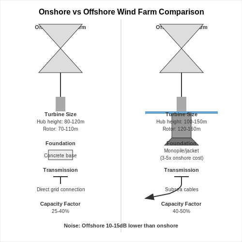
The fundamental difference between onshore and offshore wind farms lies in the wind resource profile. Offshore locations typically experience higher and more consistent wind speeds due to reduced surface roughness over water. The power output of a wind turbine scales with the cube of wind velocity:
where ρ is air density, A is swept area, v is wind velocity, and Cp is the power coefficient (Betz limit ≈ 0.59). A 10% increase in wind speed yields a 33% increase in energy production. Offshore sites commonly achieve capacity factors of 45-55%, compared to 30-40% for onshore.
Turbine Design and Scaling
Offshore turbines employ larger rotors (180-220m diameter) and taller towers (120-160m) to capture more energy from the smoother wind shear profile. The scaling laws for turbine components reveal why offshore designs diverge:
where D is rotor diameter and H is hub height. Modern offshore turbines (12-15MW) use direct-drive permanent magnet generators to reduce maintenance needs, while onshore turbines (3-6MW) often employ geared drivetrains for cost efficiency.
Installation and Infrastructure Costs
Offshore wind requires specialized installation vessels costing $$200-500k/day, with foundation expenses varying by water depth:
- Monopile: 20-30m depth, $$1.5-2.5M per unit
- Jacket: 30-50m depth, $$3-5M per unit
- Floating: >50m depth, $$8-12M per unit
Onshore projects benefit from standardized transportation and crane access, with balance-of-system costs typically 30-40% lower per MW installed.
Grid Integration Challenges
Offshore wind farms require HVDC transmission systems for distances >80km, introducing additional conversion losses (1.5-2.5% per converter station). The reactive power demand of submarine cables necessitates compensation strategies:
where C is cable capacitance and V is operating voltage. Onshore projects can typically connect via AC transmission with simpler reactive power management.
Environmental and Regulatory Factors
Offshore wind faces unique constraints from marine ecosystems and shipping lanes, requiring extensive environmental impact assessments. The noise propagation underwater follows different physics than airborne transmission:
where TL is transmission loss, r is distance in meters, and α is frequency-dependent absorption coefficient. Onshore projects must address avian impacts and community noise limits (typically 45 dB(A) at nearest dwellings).
3.3 Energy Conversion and Efficiency
Fundamentals of Energy Conversion
The conversion of energy in renewable systems is governed by the first and second laws of thermodynamics. For a system with input energy Ein, useful output Eout, and losses Eloss, the energy balance is:
Efficiency (η) quantifies the ratio of useful output to total input:
Carnot Limit and Practical Constraints
For heat engines (e.g., concentrated solar power), the maximum theoretical efficiency is bounded by the Carnot efficiency:
where TC and TH are the cold and hot reservoir temperatures (in Kelvin). Photovoltaic cells, however, are limited by the Shockley-Queisser limit (~33.7% for single-junction Si cells).
Loss Mechanisms in Renewable Systems
- Ohmic losses in conductors: Ploss = I²R
- Optical losses in solar panels (reflection, spectral mismatch)
- Mechanical losses in wind turbines (bearing friction, tip vortices)
Case Study: Grid-Tied Inverter Efficiency
A 5 kW solar inverter with 97% peak efficiency might exhibit a European weighted efficiency (ηEU) of:
Multi-Stage Conversion Systems
For hybrid systems (e.g., wind-to-hydrogen), total efficiency is the product of individual stage efficiencies:
Modern PEM electrolyzers achieve ~75% efficiency at 1 A/cm², while alkaline variants reach ~65%.
4. Principles of Hydropower Generation
Principles of Hydropower Generation
Energy Conversion in Hydropower Systems
The fundamental principle of hydropower generation lies in converting the potential and kinetic energy of flowing or falling water into mechanical energy, which is then transformed into electrical energy. The total extractable power P from a water source is derived from Bernoulli’s equation, considering elevation head h, volumetric flow rate Q, and water density ρ:
where g is gravitational acceleration (9.81 m/s²). For practical systems, efficiency η (typically 80–95% for modern turbines) must be included:
Turbine Selection and Hydrodynamic Principles
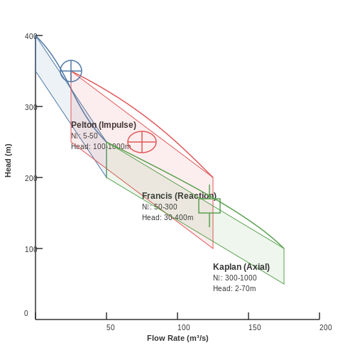
Turbine efficiency depends on the specific speed Ns, a dimensionless parameter classifying turbines based on head and flow conditions:
Key turbine types include:
- Pelton wheels: Impulse turbines for high-head (>300 m), low-flow applications.
- Francis turbines: Mixed-flow reaction turbines for medium-head (10–300 m) scenarios.
- Kaplan turbines: Axial-flow reaction turbines for low-head (<10 m), high-flow systems.
Penstock Dynamics and Loss Modeling
Penstock design critically affects system performance. Head loss hf due to friction is modeled via the Darcy-Weisbach equation:
where f is the friction factor, L and D are penstock length and diameter, and v is flow velocity. Surge pressure Δp during valve operations must also be considered:
where a is the pressure wave speed (≈1200 m/s for water) and Δv is the velocity change rate.
Grid Synchronization and Frequency Control
Modern hydropower plants use doubly-fed induction generators (DFIGs) or synchronous generators with automatic voltage regulators (AVRs) and power system stabilizers (PSS). The grid-tie condition requires:
where p is the number of poles and Nrotor is rotational speed (RPM). Frequency droop control maintains stability during load changes:
with R as the droop constant (typically 4–5% in large systems).
Environmental and Operational Constraints
Fish-friendly turbine designs now incorporate:
- Minimum flow rates to preserve aquatic ecosystems (often enforced via Q10 standards).
- Sediment bypass systems to prevent reservoir siltation.
- Bubble curtain systems to mitigate dissolved gas supersaturation.
4.2 Tidal and Wave Energy Technologies
Fundamentals of Tidal Energy Conversion
Tidal energy harnesses the gravitational interaction between the Earth, Moon, and Sun, converting the kinetic energy of tidal currents or potential energy from tidal height differences into electricity. The power density of a tidal stream can be derived from the kinetic energy flux per unit area:
where ρ is seawater density (~1025 kg/m³), A is the cross-sectional area of the turbine, and v is the flow velocity. For a tidal range system (e.g., tidal barrages), the potential energy is given by:
where Δh is the tidal height differential and g is gravitational acceleration. Modern tidal turbines achieve 40-50% efficiency, with rated velocities typically between 2.5–3.5 m/s.
Turbine Technologies and Hydrodynamic Design
Three dominant turbine architectures exist:
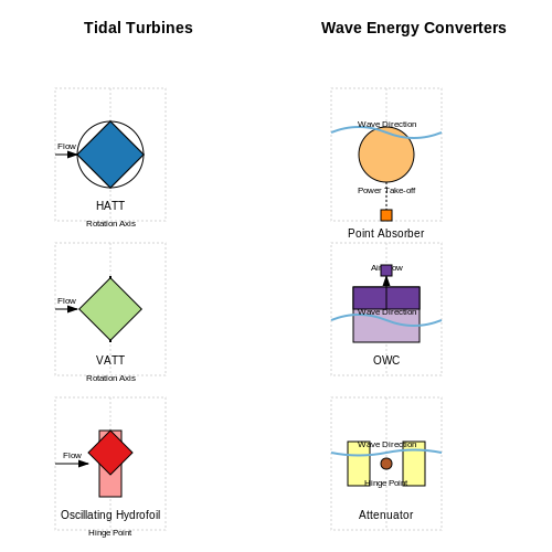
- Horizontal-axis tidal turbines (HATTs): Function similarly to wind turbines, with 3-5 blades optimized for high torque at low tip-speed ratios (λ ≈ 5-7). Blade profiles use NACA 6-series hydrofoils to minimize cavitation.
- Vertical-axis turbines (VATTs): Darrieus-type designs enable omnidirectional operation but suffer from cyclical torque fluctuations. Power coefficient (Cp) peaks around 0.35 compared to 0.45 for HATTs.
- Oscillating hydrofoils: Utilize lift-generated pitching motions to drive hydraulic systems, achieving Cp > 0.4 in experimental prototypes.
The Betz limit for tidal turbines is 59.3%, identical to wind turbines, as both operate in open-flow conditions. However, tidal devices must account for additional constraints:
where ω is angular velocity and R is rotor radius. Optimal λ values are lower than wind turbines due to higher fluid density.
Wave Energy Converter (WEC) Architectures
Wave energy systems convert the orbital motion of water particles into electricity through three primary mechanisms:
- Point absorbers: Floating buoys that drive linear or rotary generators via heave motion. The hydrodynamic response is modeled as a mass-spring-damper system:
where m includes added mass effects, b is the radiation damping coefficient, and k is hydrostatic stiffness.
- Oscillating water columns (OWCs): Capture air displacement from wave action to drive Wells turbines, which maintain unidirectional rotation despite bidirectional airflow.
- Attenuators: Multi-segment floating structures (e.g., Pelamis) that flex at hinged joints, with hydraulic rams converting relative motion into energy.
Power Take-Off (PTO) Systems
Efficient energy conversion requires tailored PTO designs:
| PTO Type | Efficiency | Application |
|---|---|---|
| Direct-drive permanent magnet generators | 85-92% | High-speed tidal turbines |
| Hydraulic accumulators | 70-80% | Wave energy converters |
| Reciprocating electro-magnetic systems | 75-85% | Oscillating hydrofoils |
Modern projects like the 398 MW Swansea Bay Tidal Lagoon and the 1.5 MW Mutriku OWC plant demonstrate commercial viability, with LCOE projections declining below $0.15/kWh for next-generation systems.
Environmental and Material Challenges
Turbine blades face cavitation erosion at tip speeds exceeding 15 m/s, requiring nickel-aluminum-bronze alloys or fiber-reinforced composites. Biofouling can reduce power output by 20% within 6 months, necessitating antifouling coatings or UV sterilization systems. Mooring systems for WECs must withstand 50-year storm conditions with peak wave heights exceeding 15 meters.
4.3 Environmental Impacts and Mitigation
Lifecycle Emissions of Renewable Energy Systems
While renewable energy systems produce negligible operational emissions, their lifecycle environmental impact must be evaluated through a cradle-to-grave analysis. Photovoltaic (PV) systems, for example, incur emissions during:
- Silicon purification and panel manufacturing
- Transportation and installation
- End-of-life recycling or disposal
The energy payback time (EPT) quantifies how long a system must operate to offset its embodied energy. For modern silicon PV:
where \(E_{\text{manufacturing}}\) is the total energy consumed during production and \(P_{\text{annual}}\) is annual energy generation. Typical EPT values range from 1-4 years for commercial PV modules.
Land Use and Ecological Disruption
Utility-scale renewables require significant land area per unit energy. The power density \( \rho \) (W/m²) varies substantially:
Comparative studies show:
- Wind farms: 1-3 W/m² (including spacing between turbines)
- Solar PV: 5-20 W/m²
- Biomass: <0.5 W/m²
Mitigation strategies include agrivoltaics (dual-use land for agriculture and PV) and offshore wind deployment to minimize terrestrial ecosystem impacts.
Material Resource Constraints
Critical materials pose supply chain risks:
| Technology | Key Materials | Recycling Rate |
|---|---|---|
| PV (CdTe) | Tellurium, Cadmium | >90% (module recovery) |
| Li-ion Batteries | Lithium, Cobalt | ~50% (current) |
Emerging circular economy approaches employ:
- Design for disassembly standards
- Hydrometallurgical recovery processes
- Material substitution (e.g., perovskite PV)
Avian and Wildlife Impacts
Wind turbines cause ~0.3 avian fatalities per GWh generated, compared to 5.2 for fossil plants when considering secondary effects like climate change. Mitigation techniques include:
- Radar-activated curtailment
- Ultraviolet lighting to deter insects (reducing prey attraction)
- Proper siting away from migration corridors
Noise and Visual Pollution
Wind turbine sound power levels follow:
where \(P_0 = 10^{-12}\) W. Modern turbines operate at ~105 dB at source, but setback regulations typically limit residential exposure to <45 dB. Aesthetic concerns are addressed through:
- Community benefit agreements
- Camouflage coloring
- Subsurface transmission lines
5. Biomass Conversion Processes
5.1 Biomass Conversion Processes
Thermochemical Conversion
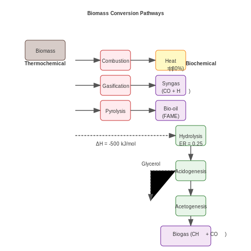
Thermochemical processes decompose biomass through heat-driven reactions, primarily classified into combustion, gasification, pyrolysis, and liquefaction. The fundamental energy balance for these processes is derived from the first law of thermodynamics:
For gasification, the equivalence ratio (ER)—defined as the actual air-to-fuel ratio divided by the stoichiometric air-to-fuel ratio—critically influences syngas composition. A typical reaction for cellulose (C6H10O5) gasification at ER = 0.3 yields:
Pyrolysis Kinetics
Pyrolysis follows Arrhenius-type kinetics, where the rate constant k is expressed as:
Key parameters:
- A: Pre-exponential factor (106–1018 s−1 for biomass)
- Ea: Activation energy (50–250 kJ/mol)
- Fast pyrolysis (500°C, 103°C/s) maximizes bio-oil yield (~70 wt%).
Biochemical Conversion
Anaerobic digestion converts organic matter into biogas (CH4 + CO2) via four stages:
- Hydrolysis: Polymers → monomers (e.g., cellulose → glucose)
- Acidogenesis: Monomers → volatile fatty acids (VFAs)
- Acetogenesis: VFAs → acetic acid, H2, CO2
- Methanogenesis: Acetate → CH4 + CO2 (ΔG° = −31 kJ/mol)
The Chen-Hashimoto model predicts methane production rate r:
where S = substrate concentration, Ks = half-saturation constant, and μm = maximum growth rate.
Physicochemical Processes
Transesterification converts lipids to biodiesel (FAME) via base-catalyzed reaction:
Optimization criteria:
- Methanol-to-oil molar ratio: 6:1–9:1
- Catalyst concentration: 0.5–2 wt%
- Reaction temperature: 60–70°C (above methanol boiling point requires pressurized systems)
System Integration
Combined heat and power (CHP) systems using biomass gasification achieve electrical efficiencies (ηel) of 25–40% and thermal efficiencies (ηth) up to 85%. The overall efficiency ηtotal is:
Advanced systems integrate carbon capture and storage (BECCS), achieving negative emissions of −0.5 to −1.0 tCO2/MWh.
5.2 Geothermal Energy Extraction Methods
Direct Steam Systems
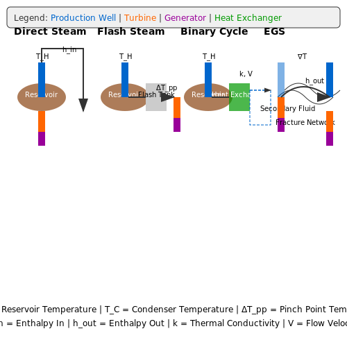
Direct steam systems exploit high-temperature geothermal reservoirs (>235°C) where steam is directly available. The steam is piped from production wells to drive turbines connected to generators. The Carnot efficiency for such systems is given by:
where TC is the condenser temperature (typically 30-50°C) and TH is the steam temperature. The Larderello field in Italy, operational since 1913, remains a prime example with 800 MW capacity.
Flash Steam Systems
For reservoirs with pressurized water at 180-235°C, flash steam systems are employed. As fluid rises, pressure drops cause rapid vaporization ("flashing"). The two-phase flow is separated, with steam directed to turbines. The specific enthalpy (h) determines extractable work:
The Cerro Prieto plant in Mexico uses this method, achieving 820 MW output. Separation efficiency critically impacts performance—modern cyclonic separators achieve >99% vapor purity.
Binary Cycle Systems
For lower-temperature resources (85-180°C), binary systems transfer heat to a secondary fluid (e.g., isobutane) with lower boiling points via heat exchangers. The Rankine cycle efficiency is optimized by the pinch point:
Chena Hot Springs in Alaska (400 kW) operates with a 57°C resource using R134a refrigerant. Recent advances in nanofluids as working fluids show 12-15% efficiency gains.
Enhanced Geothermal Systems (EGS)
EGS creates artificial reservoirs in hot dry rock (HDR) through hydraulic stimulation. The thermal power output depends on fracture network conductivity (k), reservoir volume (V), and temperature gradient (∇T):
The Soultz-sous-Forêts project in France demonstrated 1.5 MW net generation from 200°C rock at 5 km depth. Microseismic monitoring ensures fracture control within ±10 m precision.
Hybrid Systems
Co-production with fossil fuels or solar thermal input boosts efficiency. The Stillwater plant in Nevada combines 33 MW geothermal with 26 MW solar PV, reducing LCOE by 18%. Thermoeconomic optimization models balance CAPEX and exergy destruction:
where Ċinv is capital cost rate and cex is exergy unit cost.
5.3 Sustainability and Scalability
Energy Return on Investment (EROI)
The sustainability of renewable energy systems is often quantified using the Energy Return on Investment (EROI), defined as the ratio of usable energy output to the energy required to extract, refine, and deliver it. For a system to be viable, EROI must exceed a threshold value, typically around 7:1 for modern economies. The EROI for solar photovoltaics (PV) has improved significantly due to advances in manufacturing, now ranging between 10:1 and 30:1, while wind energy systems achieve 18:1 to 50:1.
Material and Land Use Constraints
Scalability is constrained by material availability, particularly for technologies like lithium-ion batteries and rare-earth magnets in wind turbines. For instance, neodymium demand for permanent magnet generators could grow by 250% by 2050. Land use efficiency also varies widely: utility-scale solar requires 3–10 acres per MW, while onshore wind needs 30–140 acres per MW, accounting for turbine spacing.
Grid Integration Challenges
High penetration of renewables introduces stability challenges due to intermittency. The capacity factor (actual output vs. maximum potential) for solar and wind typically ranges from 20–40%, necessitating storage or backup systems. Grid-scale battery storage must compensate for the temporal mismatch between supply and demand, with discharge durations currently limited to 4–12 hours for lithium-ion systems.
Technological Pathways for Scalability
Emerging solutions include:
- Perovskite solar cells with theoretical efficiencies exceeding 30% and reduced material costs
- Offshore wind farms leveraging higher wind speeds (Class 4–7) and capacity factors >50%
- Green hydrogen production via electrolysis at efficiencies approaching 80% with PEM technology
Case Study: Germany’s Energiewende
Germany’s energy transition demonstrates both successes and limitations. Renewable share reached 46% of electricity generation in 2022, but system costs exceeded €25 billion annually due to:
- Curtailement of 5.8 TWh wind energy in 2021
- Dependence on natural gas peaker plants during Dunkelflaute (low wind/solar periods)
- Transmission losses exceeding 6% for north-south power transfers
Lifecycle Analysis Framework
A comprehensive sustainability assessment must include:
Where LCCO2 is lifecycle carbon output, Ei is energy input at stage i, CIi is carbon intensity, Mi is material mass, and CFi is material carbon footprint.
6. Hybrid Renewable Energy Systems
6.1 Hybrid Renewable Energy Systems
Hybrid renewable energy systems (HRES) integrate multiple energy generation sources—typically solar, wind, hydro, and storage—to enhance reliability, efficiency, and grid stability. Unlike standalone systems, HRES leverages complementary generation profiles to mitigate intermittency, a critical challenge in renewable energy deployment.
System Architecture and Components
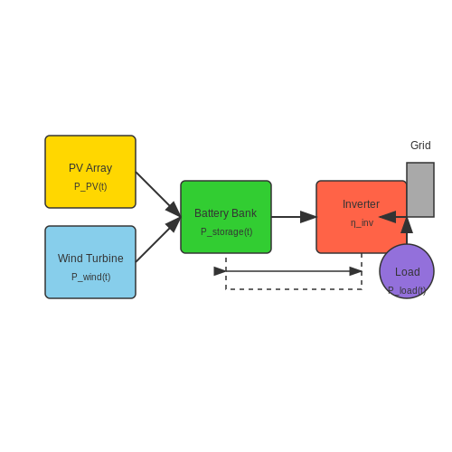
A typical HRES consists of:
- Primary generation sources (e.g., photovoltaic arrays, wind turbines, small-scale hydro).
- Energy storage systems (e.g., lithium-ion batteries, flow batteries, pumped hydro).
- Power electronics (inverters, charge controllers, maximum power point trackers).
- Control systems (rule-based, model predictive control, AI-driven optimization).
The system architecture varies based on resource availability and load requirements. For instance, a solar-wind hybrid system in a high-insolation, low-wind region may prioritize photovoltaic capacity with wind as a supplementary source.
Mathematical Modeling of Power Flow
The net power output of an HRES at time t is given by:
where:
- PPV(t) is the photovoltaic power output, modeled as:
$$ P_{PV}(t) = \eta_{PV} \cdot A \cdot G(t) \cdot (1 - 0.005(T_c(t) - 25)) $$
Here, ηPV is panel efficiency, A is array area, G(t) is solar irradiance, and Tc(t) is cell temperature.
- Pwind(t) follows the Betz-limited power curve:
$$ P_{wind}(t) = \begin{cases} 0 & v(t) < v_{cut-in} \\ \frac{1}{2} \rho A v(t)^3 C_p & v_{cut-in} \leq v(t) < v_{rated} \\ P_{rated} & v_{rated} \leq v(t) < v_{cut-out} \\ 0 & v(t) \geq v_{cut-out} \end{cases} $$
Energy Storage Sizing and Optimization
Battery capacity Cbat is determined by the autonomy period Na and depth of discharge DOD:
where Eload is daily load energy, ηbat is round-trip efficiency, and Vsys is system voltage. Advanced optimization techniques like particle swarm optimization (PSO) are often employed to minimize levelized cost of energy (LCOE).
Grid Integration and Power Electronics
HRES interfacing with the grid requires:
- Synchronous inverters for frequency and phase matching.
- Anti-islanding protection (IEEE 1547 compliance).
- Reactive power compensation (e.g., STATCOMs) for voltage regulation.
The inverter's DC-AC conversion efficiency ηinv impacts overall system performance:
Case Study: Solar-Wind-Diesel Hybrid System
A 500 kW hybrid system in Antarctica combines:
- 300 kW photovoltaic array with snow-shedding coatings.
- 150 kW vertical-axis wind turbines (operational at -40°C).
- 50 kW diesel backup with waste heat recovery.
This configuration achieves 92% renewable penetration, reducing fuel consumption by 8,000 liters/year compared to diesel-only systems.
6.2 Role of Energy Storage in Renewable Systems
Energy Storage as a Grid Stabilization Mechanism
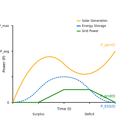
Renewable energy sources such as solar and wind are inherently intermittent, leading to supply-demand mismatches. Energy storage systems (ESS) mitigate this by decoupling generation from consumption. The instantaneous power balance equation for a grid-integrated ESS is:
where Pgrid is the net power flow, Pgen is renewable generation, Pload is demand, and PESS represents charging (negative) or discharging (positive) power. Storage systems smooth fluctuations by absorbing excess energy during surplus periods and injecting it during deficits.
Key Storage Technologies and Their Dynamics
Different storage technologies serve distinct roles based on their energy density, power density, and response time:
- Lithium-Ion Batteries: High energy density (~250 Wh/kg) and efficiency (~95%) make them ideal for short-term (minutes to hours) load shifting.
- Pumped Hydro Storage: Offers large-scale (GWh) capacity but requires geographic constraints. The round-trip efficiency is ~70-80%.
- Flywheels: Ultra-fast response (<100 ms) suits frequency regulation. Energy is stored kinetically as E = ½Iω², where I is moment of inertia and ω is angular velocity.
Mathematical Modeling of Storage Performance
The state of charge (SOC) for a battery system is governed by:
where SOC0 is the initial charge, η is charge/discharge efficiency, and Crated is rated capacity. Degradation effects, such as capacity fade, follow empirical models like:
where A is a pre-exponential factor, Ea is activation energy, DoD is depth of discharge, and z is a stress factor.
Case Study: Grid-Scale Storage in California
The Hornsdale Power Reserve in South Australia, featuring a 150 MW/194 MWh lithium-ion system, reduced grid stabilization costs by 90% by providing frequency control ancillary services (FCAS). The system’s response time of 140 ms underscores the critical role of fast-cycling storage in modern grids.
Future Directions: Hybrid Storage Systems
Combining high-energy (e.g., flow batteries) and high-power (e.g., supercapacitors) technologies optimizes cost and performance. A hybrid system’s net present value (NPV) can be evaluated via:
where r is the discount rate, and Csavings derives from avoided peaker-plant usage and reduced curtailment.
6.3 Smart Grid Technologies and Demand Response
Fundamentals of Smart Grid Architecture
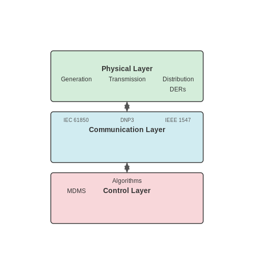
The smart grid represents an evolution of traditional power systems, integrating bidirectional communication, distributed energy resources (DERs), and advanced control algorithms. Its architecture comprises three primary layers:
- Physical Layer: Power generation, transmission, and distribution infrastructure, including renewable energy sources, energy storage, and flexible loads.
- Communication Layer: Real-time data exchange via protocols like IEC 61850, DNP3, and IEEE 1547, enabling coordination between grid components.
- Control Layer: Decision-making algorithms for optimal power flow, fault detection, and demand-side management.
Demand Response (DR) Mechanisms
DR programs dynamically adjust electricity consumption in response to supply conditions or price signals. The two primary DR strategies are:
- Price-Based DR: Consumers respond to time-varying electricity prices (e.g., Time-of-Use, Critical Peak Pricing). The demand elasticity E is given by:
where Q is demand, P is price, and subscript 0 denotes baseline values.
- Incentive-Based DR: Participants receive payments for load reductions during peak periods. Common programs include Direct Load Control and Emergency Demand Response.
Advanced Metering Infrastructure (AMI)
AMI forms the backbone of smart grid communication, consisting of:
- Smart meters with two-way communication
- Data concentrators for neighborhood aggregation
- Meter data management systems (MDMS)
The data sampling rate fs must satisfy the Nyquist criterion for accurate load profiling:
where fmax is the highest frequency component of the load waveform.
Distributed Energy Resource Management
Smart grids must coordinate diverse DERs while maintaining stability. The power balance equation for a microgrid with N DERs is:
where PDER_i is power from the ith DER, Pgrid is utility power exchange, Pload is total demand, and Ploss represents system losses.
Real-World Implementation Challenges
Practical smart grid deployments face several technical hurdles:
- Latency requirements for protection schemes (<1ms for differential protection)
- Cybersecurity threats to SCADA systems
- Interoperability between legacy and modern equipment
The IEEE 2030.5 standard provides a framework for DER integration, specifying communication protocols and data models for seamless interoperability.
7. Cost Analysis and Financial Incentives
7.1 Cost Analysis and Financial Incentives
Levelized Cost of Energy (LCOE)
The Levelized Cost of Energy (LCOE) is a fundamental metric for comparing the cost-effectiveness of different renewable energy systems. It represents the net present value of the unit cost of electricity over a system's lifetime, accounting for capital costs, operational expenses, and capacity factors. The LCOE is derived as:
Where:
- It = Initial investment in year t
- Mt = Maintenance costs in year t
- Ft = Fuel costs (if applicable, e.g., biomass)
- Et = Energy produced in year t
- r = Discount rate
- N = System lifetime (years)
For photovoltaic (PV) systems, Ft is typically zero, while wind turbines incur periodic maintenance costs. The discount rate r heavily influences LCOE, with higher rates penalizing capital-intensive technologies like nuclear or offshore wind.
Net Present Value (NPV) and Internal Rate of Return (IRR)
Investors evaluate renewable projects using Net Present Value (NPV) and Internal Rate of Return (IRR). NPV calculates the profitability of a project by discounting future cash flows:
Where Ct is the net cash flow in year t. A positive NPV indicates a viable investment. IRR, the discount rate that zeroes NPV, provides a percentage return metric. Renewable projects typically require an IRR exceeding 8–12% to attract private capital.
Financial Incentives and Policy Mechanisms
Governments deploy multiple instruments to accelerate renewable adoption:
- Feed-in Tariffs (FiTs): Guaranteed fixed prices for renewable electricity, ensuring long-term revenue stability.
- Power Purchase Agreements (PPAs): Contracts between generators and off-takers (utilities/corporations) locking in prices for 10–25 years.
- Tax Credits: Direct reductions in tax liability (e.g., U.S. Investment Tax Credit (ITC) covering 26–30% of solar project costs).
- Renewable Portfolio Standards (RPS): Mandates requiring utilities to source a percentage of power from renewables.
Case Study: German Energiewende
Germany’s Energiewende policy combined FiTs with grid priority for renewables, driving solar PV capacity from 5.4 GW in 2005 to 59 GW in 2022. However, FiTs led to €29 billion/year in subsidies, prompting a shift to competitive auctions in 2017.
Sensitivity Analysis and Risk Assessment
Renewable projects face uncertainties in:
- Capital Expenditure (CapEx): PV module prices fell 82% (2010–2020), but supply chain disruptions can cause volatility.
- Energy Yield: Wind/solar resource variability affects revenue. Monte Carlo simulations quantify probabilistic LCOE ranges.
- Policy Risk: Sudden subsidy cuts (e.g., Spain’s 2013 retroactive FiT reduction) can destabilize returns.
A robust sensitivity analysis varies key inputs (discount rate, CapEx, capacity factor) by ±20% to test project resilience. Tools like NREL’s System Advisor Model (SAM) automate these assessments.
Emerging Trends: Corporate PPAs and Green Bonds
Corporate PPAs (e.g., Google, Amazon) now drive ~25% of global renewable capacity additions, offering fixed prices without government subsidies. Green bonds, exceeding $1 trillion in cumulative issuance since 2007, lower financing costs by earmarking funds for sustainable projects.
7.2 Regulatory Frameworks and Standards
International Standards for Renewable Energy Integration
Renewable energy systems must comply with international standards to ensure grid stability, safety, and interoperability. The International Electrotechnical Commission (IEC) and the Institute of Electrical and Electronics Engineers (IEEE) are the primary bodies governing these standards. Key standards include:
- IEC 61400 (Wind Turbines) – Covers design, testing, and certification of wind energy systems.
- IEC 61724 (Photovoltaic System Performance) – Defines monitoring and reporting metrics for PV systems.
- IEEE 1547 (Interconnection Standards) – Specifies technical requirements for connecting distributed energy resources (DERs) to the grid.
These standards ensure that renewable energy systems operate efficiently while maintaining grid reliability. For example, IEEE 1547-2018 introduces advanced inverter functionalities such as voltage and frequency ride-through, which are critical for modern grid support.
National and Regional Regulatory Policies
Regulatory frameworks vary by country but generally focus on incentivizing renewable adoption while ensuring grid compatibility. Key policies include:
- Feed-in Tariffs (FiTs) – Guarantee fixed payments for renewable energy fed into the grid, encouraging investment.
- Renewable Portfolio Standards (RPS) – Mandate a minimum percentage of energy generation from renewables.
- Net Metering – Allows consumers to offset their electricity bills with surplus renewable generation.
In the European Union, the Renewable Energy Directive (RED II) sets binding targets for 32% renewable energy by 2030, with strict sustainability criteria for biofuels and bioliquids.
Grid Compliance and Power Quality
Renewable energy systems must adhere to strict power quality standards to prevent grid disturbances. Key parameters include:
Grid operators enforce these limits through EN 50160 (Europe) and ANSI C84.1 (North America). Advanced inverters use real-time control algorithms to maintain compliance under varying generation conditions.
Case Study: Germany’s Energiewende
Germany’s transition to renewables (Energiewende) provides a practical example of regulatory success. Key measures include:
- EEG (Renewable Energy Sources Act) – Prioritizes renewable energy feed-in and guarantees compensation.
- Grid Expansion Acceleration Act – Fast-tracks transmission infrastructure to accommodate decentralized generation.
These policies have enabled Germany to achieve over 40% renewable electricity penetration, demonstrating the effectiveness of well-designed regulatory frameworks.
Emerging Standards for Energy Storage
With the rise of battery storage, new standards are being developed to address safety and performance:
- UL 9540 (Energy Storage Systems) – Covers fire safety and system performance.
- IEC 62933 (Grid-Connected Storage) – Defines testing and operational requirements.
These standards are critical for ensuring that storage systems integrate seamlessly with renewable generation while mitigating risks such as thermal runaway in lithium-ion batteries.
7.3 Future Prospects and Innovations
Next-Generation Photovoltaics
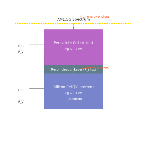
The Shockley-Queisser limit of ~33.7% for single-junction solar cells has driven research into multi-junction architectures. Recent advances in perovskite-silicon tandem cells have achieved certified efficiencies exceeding 32.5% under AM1.5G conditions. The voltage matching condition for tandem cells requires:
where Vtop and Vbottom represent the open-circuit voltages of the subcells, and Rs accounts for series resistance losses. Emerging quantum dot photovoltaics show promise through hot-carrier extraction, with theoretical modeling predicting potential efficiencies above 45% using tailored bandgap engineering.
Advanced Wind Energy Systems
Airborne wind energy (AWE) systems utilizing tethered drones or kites can access higher-altitude winds with power densities 5-8 times greater than conventional turbines. The Betz-optimal power extraction for crosswind kite systems follows:
where CL and CD represent the lift and drag coefficients of the airfoil. Recent prototypes like X-Wind's 500 kW system demonstrate capacity factors exceeding 60% in field tests.
Nuclear Fusion Breakthroughs
Inertial confinement fusion at the National Ignition Facility achieved Q>1 (energy gain) in 2022, while tokamak designs benefit from high-temperature superconductors. The Lawson criterion for net power:
shows how advanced superconducting magnets enabling higher plasma densities (n) and confinement times (τE) are critical. SPARC and ITER projects aim for Q≥10 by 2030.
Grid-Scale Storage Innovations
Solid-state batteries with lithium metal anodes are approaching 500 Wh/kg energy densities, while redox flow batteries benefit from novel organic electrolytes. The round-trip efficiency (ηrt) for a vanadium flow battery is given by:
Recent advances in catalytic hydrogen storage achieve volumetric densities of 50 g/L at moderate pressures using metal-organic frameworks (MOFs).
Artificial Photosynthesis
Molecular catalysts for water splitting now achieve turnover frequencies >106 with quantum yields approaching 80% for visible light. The overpotential (η) for the oxygen evolution reaction follows:
where ENernst = 1.23 V at STP. Cobalt-phosphate co-catalysts on hematite photoanodes demonstrate sustained operation at 10 mA/cm2 with minimal degradation.
8. Key Research Papers and Articles
8.1 Key Research Papers and Articles
- Power electronics in renewable energy systems and smart grid — Chapter 1, EnEnERgy ViRonmEnt, PowER ELECtRoniCs, REnEwAbLE EnERgy systEms, And smARt gRid 1 bimal K. bose and Fei (Fred) wang 1.1 Introduction 1 1.2 Energy 1 1.3 Environment 4 1.3.1 Environmental Pollution by Fossil Fuels 4 1.3.2 Climate Change or Global Warming Problems 7 1.3.3 Several Beneficial Effects of Climate Change 11
- Renewable energy systems: Comparisons, challenges and barriers ... — Variable renewable energy (VREs) is a term that describes a type of renewable energy, such as solar and wind and their highly intermittent nature when compared to other RERs [116, 127]. Eenergy storage systems ESSs have been largely recognized as the ultimate solution to smoothing out the RERs power generation scheme.
- Journal of Renewable Energy - Wiley Online Library — 1. Introduction. In order to mitigate the current global energy demand and environmental challenges associated with the use of fossil fuels, there is a need for better energy alternatives and robust energy storage systems that will accelerate decarbonization journey and reduce greenhouse gas emissions and inspire energy independence in the future.
- Smart investigation of artificial intelligence in renewable energy ... — Based on the literature, several research studies have been conducted in different engineering and science fields with focus on AI applications for prediction and classification purposes (Zendehboudi et al., 2018, Seyyedattar et al., 2020).In this regard, some researchers have focused on leveraging AI in different renewable energy systems, from electrical and power systems (Zhou et al., 2022 ...
- Integration of Renewable Energy in Microgrids and Smart Grids in ... — The economic viability of a hybrid renewable energy system (HRES) is achieved when the levelized COE (LCOE) does not exceed the price of imported energy. The computational results suggest that in Finland, the grid parity of an HRES is obtained at electricity prices between 17 and 29 €c kWh −1 , including transfer charges and taxes. [ 6 ]
- Comprehensive study of the artificial intelligence applied in renewable ... — This energy revolution using sustainable RE technologies has the key features to be implemented in the power sector, including controlling electricity costs [12], developing the adaptability and stability of energy systems [13], replacing old infrastructure, reducing CO 2 emissions, providing consistent power support to remote areas, and preventing changes in the atmospheric environment [14].
- Update on current approaches, challenges, and prospects of modeling and ... — The development of energy sources that are renewable and sustainable is a critical component in achieving the United Nations' sustainable development goals [[1], [2], [3]].Although the development of energy systems with renewable and sustainable sources in many industrialized economies is the first step towards attaining global environmental sustainability, studies have shown that meeting the ...
- Thermal Analysis of Power Electronic Devices Used in Renewable Energy ... — International Journal of Engineering Research and Technology, 2020. The paper presents the results of an investigation was the general purpose of characterization and thermo-graphic evaluation electronic power semiconductor devices used in cyclo converters subjected to electric charges. ... Renewable Energy Systems Alhussein Albarbar Canras ...
- Power Electronics for Renewable Energy Systems, Transportation and ... — FOR RENEWABLE ENERGY SYSTEMS, TRANSPORTATION AND INDUSTRIAL APPLICATIONS Editedby Haitham Abu-Rub TexasA&MUniversityatQatar,Doha,Qatar Mariusz Malinowski WarsawUniversityofTechnology,Warsaw,Poland Kamal Al-Haddad ÉcoledeTechnologieSupérieure,Montreal,Canada
- Effective optimal control of a wind turbine system with hybrid energy ... — This research paper discusses a wind turbine system and its integration in remote locations using a hybrid power optimization approach and a hybrid storage system. Wind turbine systems ...
8.2 Recommended Books and Textbooks
- Renewable and Efficient Electric Power Systems - Chegg — COUPON: RENT Renewable and Efficient Electric Power Systems 2nd edition (9781118140628) and save up to 80% on 📚textbook rentals and 90% on 📙used textbooks. Get FREE 7-day instant eTextbook access!
- Renewable and Efficient Electric Power Systems, 2nd Edition — A solid, quantitative, practical introduction to a wide range of renewable energy systems—in a completely updated, new edition The second edition of Renewable and Efficient Electric Power Systems provides a solid, quantitative, practical introduction to a wide range of renewable energy systems. For each topic, essential theoretical background is introduced, practical engineering ...
- Power Electronics in Energy Conversion Systems — The book includes detailed discussions of power converters for energy conversion techniques in renewable energy systems, grid-interactive inverters, and motor-drives. Written by a seasoned educator, Power Electronics in Energy Conversion Systems contains exclusive topics and features hundreds of helpful illustrations.
- Renewable and Efficient Electric Power Systems - Booktopia — The second edition of Renewable and Efficient Electric Power Systems provides a solid, quantitative, practical introduction to a wide range of renewable energy systems. For each topic, essential theoretical background is introduced, practical engineering considerations associated with designing systems and predicting their performance are provided, and methods for evaluating the economics of ...
- Ee - Books — BOOKS EEE EEE NEXT > D,S. Kirschen - Power Systems: Fundamental Concepts and the Transition to Sustainability O.D. Doleski - Handbook of Electrical Power Systems N. Mohan - Electric Power Systems with Renewables D.R. Patrick - Electrical Power Systems Technology M.A. Rosen - Battery Technology J. Twidell - Renewable Energy Resources
- PDF Renewable Energy Engineering — Renewable Energy Engineering Provides a quantitative yet accessible overview of renewable energy engineering practice and the technologies that will transform our energy supply systems over the coming years. Covering wind, hydro, solar thermal, photovoltaic, ocean and bioenergy, the text is suitable for engineer-ing undergraduates as well as graduate students from other numerate degrees. The ...
- Renewable and Efficient Electric Power Systems|Hardcover — The book covers foundational knowledge of electric power, up through current developments and future prospects for renewable energy. The update significantly expands core content to address topics such as energy efficiency, smart grids, energy storage, and microgrids.
- Energy Storage Devices for Renewable Energy-Based Systems — The book is also intended to be used as a textbook for masters and doctoral students who want to enhance their knowledge and understanding the concepts of renewable energy sources and state-of-the-art ESDs.
- Renewable and Efficient Electric Power Systems | Wiley — This is a comprehensive textbook for the new trend of distributed power generation systems and renewable energy sources in electric power systems. It covers the complete range of topics from fundamental concepts to major technologies as well as advanced topics for power consumers. An Instructors Manual presenting detailed solutions to all the problems in the book is available from the Wiley ...
- Renewable and Efficient Electric Power Systems — This book has been written primarily as a textbook for new courses on renew-able and efficient electric power systems. It has been designed to encourage self-teaching by providing numerous completely worked examples throughout.
8.3 Online Resources and Databases
- Lesson 8: Applied Renewable Energy Technologies — 8.0 Overview 8.1 Renewable Energy Basics 8.2. Building Integrated Solar Energy Technologies 8.3. Solar Thermal Electric Power Generation 8.4. Utility Scale Geothermal Energy Systems 8.5. Wind Energy Applications and Technologies 8.6. Bio-mass Fueled Combined Heat and Power Systems 8.7. Environmental Impact of Renewable Energy Summary & Activities
- Power electronics technologies for renewable energy sources — Power electronics—Key technology for renewable energy systems—Status and future. In 2013 3rd International Conference on Electric Power and Energy Conversion Systems, EPECS 2013 (pp. 0-5).
- Transition to renewable energy systems [electronic resource] — Transition to Renewable Energy Systems provides specific insights for energy engineers, process engineers, chemists, and physicists, as well as a sufficiently broad scope to be able to understand the challenges, opportunities and implications of a transition to renewable energy systems so that strategies can be cast. (source: Nielsen Book Data)
- AI for Power Electronics and Renewable Energy Systems — This reference book systematically treats the applications of AI in power electronics and renewable energy systems. The book begins with an introduction to AI in power systems, then subsequent chapters cover the use of AI for electric machine fault diagnosis, for power electronic reliability, design, and control, in dual-active-bridge converters; AI for distribution network voltage control ...
- PDF Renewable Energy Engineering — Renewable Energy Engineering Fully revised and updated, the second edition of Renewable Energy Engineering provides students with a quantitative and accessible introduc-tion to the renewable technologies at the heart of efforts to build a sustain-able future. Key features include new chapters on essential topics in energy storage, off-grid systems, microgrids and community energy; revised chap ...
- EE8703 - Renewable Energy Systems | PDF | Energy Development | Solar Power — EE8703 - Renewable Energy Systems - Free ebook download as PDF File (.pdf), Text File (.txt) or read book online for free.
- PDF Advanced Power Electronic Interfaces for Distributed Energy Systems — Because of the similar functions of these power electronics capabilities, the development of an advanced power electronic interface (APEI) that is scalable to meet different power requirements, with modular design, lower cost, and improved reliability, will improve the overall cost and durability of distributed and renewable energy systems.
- Power Electronics in Renewable Energy Systems and Smart Grid ... — Summary This book is an advanced approach to power electronics specifically in terms of renewable energy systems and smart grid. The fourteen chapters are updated and extended versions of the invited papers in the Proc. IEEE special issue of November 2017, contributed by a group of invited authors who are international authorities in their field.
- PDF An Overview of Distributed Energy - National Renewable Energy ... — Further, online systems can be used to coordinate electronic payment, manage forms, and transfer data to internal databases. Through these services, online application systems can facilitate all of the improvements discussed in Section 1.2.2.
- Front Matter - Wiley Online Library — Highly efficient and reliable power electronic systems that convert and process electrical energy from one form to another are critical for smart grid and renewable energy systems.