Mixing and Frequency Translation
1. Definition and Basic Principles
Mixing and Frequency Translation: Definition and Basic Principles
Fundamental Concept of Mixing
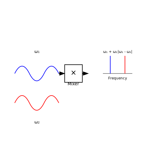
Mixing, in the context of signal processing and communications, refers to the process of combining two or more signals to produce new frequency components. The core mechanism relies on nonlinear or time-varying systems, where the interaction between input signals generates sum and difference frequencies. Mathematically, if two signals x₁(t) = A₁cos(ω₁t) and x₂(t) = A₂cos(ω₂t) are mixed, the output y(t) includes components at ω₁ + ω₂ and |ω₁ - ω₂|.
Nonlinearity and Frequency Translation
Frequency translation occurs due to the nonlinear behavior of mixers, often implemented using diodes, transistors, or analog multipliers. A square-law characteristic, typical in nonlinear devices, ensures the generation of intermodulation products. For a nonlinear system with y(t) = a₁x(t) + a₂x²(t), applying two sinusoidal inputs results in:
Practical Mixer Topologies
Common mixer implementations include:
- Diode Ring Mixers: Utilize four diodes in a ring configuration for balanced operation, suppressing carrier leakage.
- Gilbert Cell Mixers: Active mixers using differential transistor pairs for high linearity and gain.
- Passive FET Mixers: Leverage transistor switching for low-noise applications.
Image Rejection and Sideband Suppression
Mixing inherently produces both sum and difference frequencies. In receivers, this leads to the image frequency problem, where unwanted signals at ω₀ ± 2ωIF interfere with the desired signal. Techniques like image-reject mixers (e.g., Hartley or Weaver architectures) use phase cancellation to suppress these artifacts.
Applications in Modern Systems
Frequency translation is pivotal in:
- Heterodyne Receivers: Shifting RF signals to intermediate frequencies (IF) for easier amplification and filtering.
- Software-Defined Radios (SDR): Enabling flexible signal processing through digital mixing.
- Frequency Synthesizers: Generating stable local oscillator (LO) signals for phase-locked loops (PLLs).
Mathematical Derivation: Ideal Multiplier Mixer
For an ideal multiplier mixer with inputs s(t) = cos(ωₛt) (signal) and LO(t) = cos(ωₗₒt) (local oscillator), the output is:
This confirms the generation of upper and lower sidebands at ωₛ ± ωₗₒ.
1.2 Importance in Communication Systems
Frequency translation through mixing is a cornerstone of modern communication systems, enabling efficient signal processing, multiplexing, and interference mitigation. The ability to shift signals between frequency bands allows for simultaneous transmission of multiple channels, adherence to regulatory spectral allocations, and optimization of hardware performance.
Spectrum Utilization and Channelization
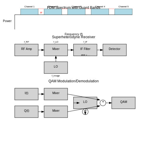
In wireless communications, the electromagnetic spectrum is a finite resource. Mixing facilitates frequency-division multiplexing (FDM), where multiple baseband signals are upconverted to distinct carrier frequencies for simultaneous transmission. For a set of N signals with bandwidth B, the total required bandwidth after mixing is:
where Δf is the guard band between channels. This principle underpins systems like FM radio, satellite transponders, and cellular networks.
Image Rejection and Superheterodyne Architectures
Mixing introduces image frequencies at fLO ± fIF, necessitating careful filtering. The superheterodyne receiver, developed by Edwin Armstrong in 1918, leverages this by:
- Downconverting the RF signal to a fixed intermediate frequency (IF)
- Applying gain and filtering at IF to reject adjacent channels
- Using double or triple conversion to mitigate image interference
The image rejection ratio (IRR) quantifies mixer performance:
Modulation and Demodulation
Mixing enables coherent modulation schemes by multiplying baseband signals with a carrier. For quadrature amplitude modulation (QAM):
where I(t) and Q(t) are in-phase and quadrature components. Synchronous demodulation recovers these components through a second mixing stage with phase-locked local oscillators.
Practical Constraints and Trade-offs
Nonlinearities in mixers generate spurious products:
where m, n are integers. System designers must balance:
- Conversion loss/gain
- Noise figure degradation
- Port-to-port isolation
- DC power consumption
Modern integrated solutions like Gilbert cell mixers address these challenges through active designs with improved linearity and port isolation.
Emerging Applications
Millimeter-wave 5G systems exploit mixing for beamforming and massive MIMO, while software-defined radios (SDRs) use digital mixing for reconfigurable frequency planning. Quantum communication systems similarly rely on frequency conversion to interface optical and microwave qubits.
1.3 Key Mathematical Foundations
Nonlinear Mixing and Trigonometric Identities
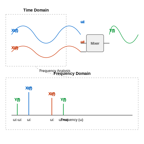
Frequency mixing relies on the nonlinear interaction between two signals, typically achieved through multiplication. Consider two sinusoidal signals, x₁(t) = A₁ cos(ω₁t) and x₂(t) = A₂ cos(ω₂t). When these signals are multiplied, the result is:
Applying the trigonometric product-to-sum identity:
We obtain the frequency-translated components:
This demonstrates how multiplication generates sum and difference frequencies, a fundamental principle in mixers.
Time-Domain vs. Frequency-Domain Analysis
In the time domain, mixing is represented as a product of signals. However, in the frequency domain, it corresponds to a convolution of their spectra. For signals X₁(f) and X₂(f), the output spectrum is:
This convolution shifts the input spectrum by ±f₂, producing sidebands at f₁ ± f₂. Practical mixers often exhibit higher-order nonlinearities, leading to additional harmonics (2f₁, 2f₂, f₁ ± 2f₂, etc.).
Phase and Amplitude Considerations
Real-world mixers introduce phase noise and amplitude imbalances. If the input signals have phase offsets ϕ₁ and ϕ₂, the output becomes:
Amplitude imbalance occurs when the mixer’s conversion gain differs for upper and lower sidebands. This is quantified as:
where G_+ and G_- are the gains at ω₁+ω₂ and ω₁-ω₂, respectively.
Intermodulation Distortion
Nonlinear systems generate intermodulation products (IMPs) when multiple tones are present. For two tones f₁ and f₂, third-order IMPs appear at 2f₁ - f₂ and 2f₂ - f₁. The output power of these products grows with a slope of 3:1 relative to the input power, leading to compression at high signal levels.
where IIP3 is the third-order intercept point, a key figure of merit for mixer linearity.
Conversion Loss and Noise Figure
Passive mixers exhibit conversion loss, defined as the ratio of desired output power to input power:
Noise figure (NF) accounts for both conversion loss and added noise:
where Tmixer is the mixer’s noise temperature and T0 = 290 K.
Image Rejection and Quadrature Mixing
Single-sideband mixing requires suppression of the image frequency. An ideal quadrature mixer combines in-phase (I) and quadrature (Q) components to cancel the image:
Image rejection ratio (IRR) quantifies performance:
Imperfections in phase (∆ϕ) and amplitude (∆A) balance degrade IRR:
2. Passive vs. Active Mixers
2.1 Passive vs. Active Mixers
Fundamental Operating Principles
Mixers perform frequency translation by multiplying two input signals, typically a radio frequency (RF) and a local oscillator (LO) signal. The mathematical representation of this operation is:
where k is the conversion gain or loss factor. This multiplication produces sum and difference frequencies at the output, enabling both upconversion and downconversion applications.
Passive Mixer Architectures
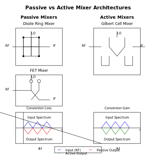
Passive mixers utilize nonlinear devices without DC power consumption. The most common implementations include:
- Diode ring mixers: Employ four diodes in a ring configuration, offering good isolation and handling high power levels
- FET mixers: Use the nonlinear resistance characteristics of field-effect transistors
- Balanced transformers: Provide inherent port-to-port isolation through symmetrical designs
The conversion loss Lc of a passive mixer is given by:
where PRF and PIF are the available powers at the RF and intermediate frequency ports respectively.
Active Mixer Topologies
Active mixers incorporate gain elements and require DC power. The Gilbert cell mixer dominates modern implementations due to its excellent balance and conversion gain:
where gm is the transconductance of the input stage and RL is the load resistance. Key advantages include:
- Positive conversion gain rather than loss
- Better port-to-port isolation
- Lower LO drive requirements
Performance Comparison
The noise figure NF of passive and active mixers differs fundamentally:
where F is the noise factor of the active devices. Linearity metrics (IIP3, P1dB) typically favor passive mixers at high signal levels, while active mixers excel in low-power applications.
Practical Implementation Considerations
In modern RF systems, the choice between passive and active mixers involves tradeoffs:
- Frequency range: Passive mixers often operate over broader bandwidths
- Power consumption: Active mixers require DC bias but may reduce overall system power by eliminating subsequent amplification
- Integration: Active mixers are more amenable to monolithic integration in CMOS/BiCMOS processes
For millimeter-wave applications above 30 GHz, active mixers dominate due to their ability to compensate transmission line losses through gain. Below 6 GHz, passive mixers remain competitive in many high-performance applications.
2.2 Single-Balanced and Double-Balanced Mixers
Fundamental Operation of Balanced Mixers
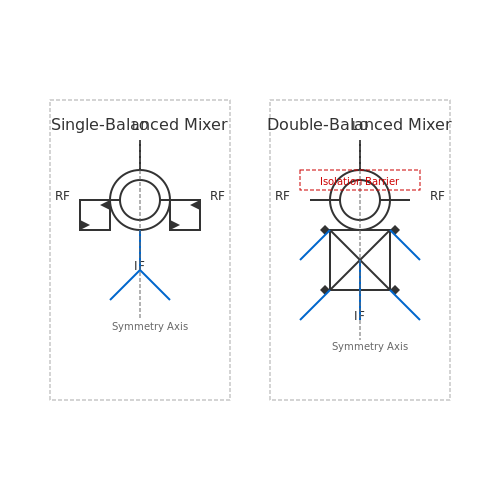
Balanced mixers suppress unwanted mixing products through symmetrical circuit topologies. The key distinction between single-balanced and double-balanced configurations lies in their port-to-port isolation and spurious rejection capabilities. Both architectures rely on diode or transistor switching action modulated by the local oscillator (LO) signal.
where sLO(t) represents the LO switching function and k is the mixer conversion constant.
Single-Balanced Mixer Topology
A single-balanced mixer provides isolation between either the LO-RF ports or LO-IF ports, but not both. The most common implementation uses a transformer-coupled diode ring with center-tapped LO injection:
Key characteristics include:
- LO suppression at IF port: Typically 20-30 dB rejection
- Conversion loss: 6-8 dB for diode-based designs
- Spurious response: Rejects even-order LO harmonics
Double-Balanced Mixer Architecture
The double-balanced configuration provides superior isolation between all three ports (LO-RF-IF) through full symmetry. The classic diode ring mixer exemplifies this topology:
Performance advantages include:
- Port-to-port isolation: >35 dB typical
- Wide bandwidth: Maintains performance over octave spans
- Spurious rejection: Suppresses both even and odd LO harmonics
where n and m are harmonic integers of LO and RF signals respectively.
Practical Implementation Considerations
Modern mixer designs often employ Gilbert cell topologies in IC implementations. Critical parameters include:
| Parameter | Single-Balanced | Double-Balanced |
|---|---|---|
| Conversion Loss | 6-8 dB | 7-9 dB |
| LO-RF Isolation | 20-30 dB | 35-45 dB |
| 1 dB Compression | +5 dBm | +10 dBm |
Diode vs. Active Mixers
While diode mixers dominate high-frequency applications (>1 GHz), active mixers provide conversion gain at lower frequencies. The choice depends on:
- Noise figure requirements
- DC power constraints
- Linearity specifications
Advanced Topics in Balanced Mixers
Recent developments include:
- Image-reject mixers: Hartley and Weaver architectures
- Subharmonic mixers: Using LO harmonics for mmWave applications
- Monolithic implementations: SiGe and GaAs IC solutions
2.3 Image Rejection and Port Isolation
Image Frequency and Mixer Spurious Responses
In a heterodyne receiver, the mixer translates both the desired RF signal at frequency fRF and its image at fimage = fLO ± fIF (with sign depending on high-side or low-side injection) to the same intermediate frequency (IF). The image rejection ratio (IRR) quantifies a receiver's ability to suppress this unwanted signal:
where Pimage and Pdesired are the powers of the image and desired signals at the IF output. For a single-mixer stage with no filtering, IRR is typically limited to 15-25 dB due to phase and amplitude imbalances in practical quadrature networks.
Port Isolation in Mixer Topologies
Mixer port isolation—specified as LO-RF, LO-IF, and RF-IF isolation—determines signal leakage between ports. Poor isolation causes:
- LO leakage to the RF port, which may radiate back through the antenna
- RF feedthrough to the IF port, reducing dynamic range
- Self-mixing where leaked LO reflects and re-enters the mixer
Double-balanced mixers using diode rings or Gilbert cells achieve 30-50 dB port isolation through symmetric cancellation. The LO-RF isolation for an ideal Gilbert cell mixer is:
where gm is the transconductance and ZIF is the IF load impedance.
Image-Reject Mixer Architectures
Two advanced techniques overcome image problems:
Hartley Architecture
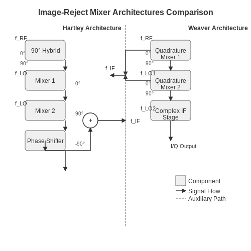
Uses a 90° hybrid coupler and two mixers with LO phases shifted by 90°. The IF outputs are summed after one branch undergoes an additional 90° phase shift, canceling the image through constructive/destructive interference.
Weaver Architecture
Employs quadrature mixing in two stages—first to a complex IF, then to baseband—eliminating the need for analog phase-shift networks. Theoretically provides infinite IRR with perfect quadrature, though limited to ~60 dB in practice by component mismatches.
where ε is the amplitude imbalance and Δφ is the phase error from quadrature.
Practical Considerations
In monolithic implementations, IRR > 40 dB requires:
- On-chip RC-CR quadrature networks with < 0.5° phase error
- Transistor matching better than 1% in Gilbert cell quads
- Differential layout with common-centroid geometries
Measured data from a 28 nm CMOS receiver shows IRR degradation versus frequency due to parasitic phase mismatches:
3. Upconversion and Downconversion
3.1 Upconversion and Downconversion
Frequency translation is a fundamental operation in communication systems, radar, and signal processing, enabling signals to be shifted to different frequency bands for efficient transmission, filtering, or demodulation. The two primary processes are upconversion (shifting a signal to a higher frequency) and downconversion (shifting a signal to a lower frequency). Both rely on nonlinear mixing to achieve frequency translation.
Mathematical Basis of Frequency Translation
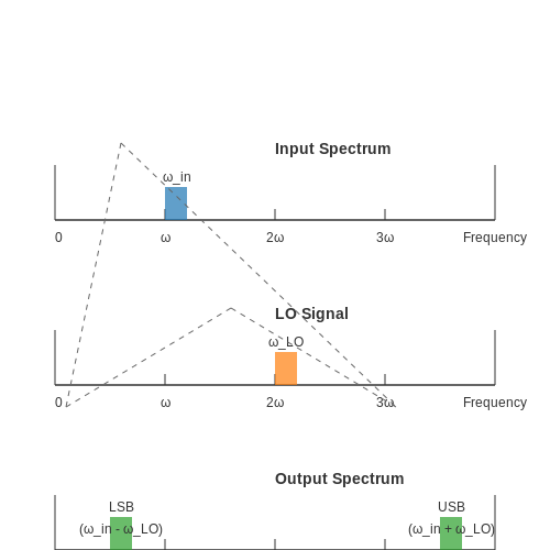
Mixing is achieved by multiplying the input signal with a local oscillator (LO) signal. Consider an input signal x(t) and an LO signal cos(ωLOt):
The product of these signals generates sum and difference frequencies due to the trigonometric identity:
This results in two components: the upper sideband (USB) at ωin + ωLO and the lower sideband (LSB) at ωin − ωLO.
Upconversion
Upconversion shifts a baseband or intermediate frequency (IF) signal to a higher carrier frequency. This is essential in transmitters to match the signal to the allocated transmission band. For example, in RF communications, voice signals (typically below 20 kHz) are upconverted to MHz or GHz ranges for wireless transmission.
The process involves:
- Multiplying the input signal with an LO signal at the desired carrier frequency.
- Filtering out the unwanted sideband (either USB or LSB) to avoid spectral redundancy.
In practice, image rejection mixers or single-sideband (SSB) modulation techniques are used to suppress the undesired sideband.
Downconversion
Downconversion translates a high-frequency signal (e.g., RF) to a lower intermediate frequency (IF) or baseband for easier processing. This is crucial in receivers where high-frequency signals must be demodulated or digitized.
The process includes:
- Mixing the RF signal with an LO to produce sum and difference frequencies.
- Filtering to retain only the desired IF component (typically the difference frequency).
Two common downconversion methods are:
- Homodyne (Direct-Conversion): The LO frequency equals the carrier frequency, converting the signal directly to baseband (DC).
- Heterodyne: The LO is offset from the carrier, producing an IF signal for further processing.
Practical Considerations
Non-ideal effects in frequency translation include:
- LO leakage: Unwanted feedthrough of the LO signal into the output.
- Image frequency interference: In downconversion, signals at ωLO ± ωIF can alias to the same IF, requiring image-reject filters.
- Phase noise: LO phase instability introduces jitter in the translated signal.
Advanced architectures like quadrature mixing (using I/Q signals) mitigate these issues by enabling complex frequency translation and sideband suppression.
Heterodyne and Homodyne Architectures
Fundamental Principles
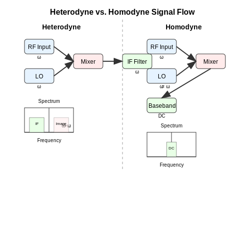
Heterodyne and homodyne architectures are foundational techniques in frequency translation, enabling the downconversion or upconversion of signals in communication systems. The core distinction lies in whether an intermediate frequency (IF) is used (heterodyne) or if the signal is directly converted to baseband (homodyne). Both methods rely on the principle of mixing, where a local oscillator (LO) signal is multiplied with the input signal to produce sum and difference frequencies.
The product yields:
Heterodyne Architecture
The heterodyne architecture employs an intermediate frequency (IF) stage, allowing for easier filtering and amplification before final downconversion to baseband. This method is widely used in superheterodyne receivers, where the RF signal is first mixed with an LO to produce an IF signal, typically at a fixed frequency. Key advantages include:
- Improved selectivity due to fixed IF filters.
- Reduced LO leakage since the LO frequency is offset from the RF.
- Better image rejection through careful choice of IF and filtering.
The primary challenge is image frequency interference, where a signal at \( f_{RF} = f_{LO} + f_{IF} \) or \( f_{RF} = f_{LO} - f_{IF} \) can alias into the IF band. This is mitigated using image-reject mixers or high-Q preselect filters.
Homodyne (Direct-Conversion) Architecture
In homodyne systems, the LO frequency is set equal to the RF carrier frequency, directly translating the signal to baseband (DC). This eliminates the need for an IF stage, simplifying the receiver chain. However, homodyne architectures face critical challenges:
- DC offsets due to LO self-mixing or component mismatches.
- I/Q imbalance causing distortion in quadrature demodulation.
- Flicker noise (1/f noise) degrading low-frequency signal integrity.
Despite these issues, homodyne receivers are prevalent in modern wireless systems (e.g., WiFi, 5G) due to their compact design and lower power consumption compared to heterodyne systems.
Practical Implementation Considerations
The choice between heterodyne and homodyne architectures depends on application-specific trade-offs:
- Heterodyne: Preferred for high-performance systems (e.g., radar, satellite comms) where selectivity and dynamic range are critical.
- Homodyne: Favored in integrated circuits (ICs) for consumer electronics due to lower component count and power efficiency.
Advanced variants like low-IF architectures blend both approaches, using a low intermediate frequency (e.g., a few MHz) to mitigate DC offsets while avoiding complex image rejection.
Case Study: Software-Defined Radio (SDR)
Modern SDRs often employ a hybrid approach, leveraging a heterodyne front-end for initial downconversion followed by digital homodyne processing. For example, an RF signal at 2.4 GHz might be mixed to a 70 MHz IF, digitized, and then digitally downconverted to baseband using numerically controlled oscillators (NCOs). This combines the analog robustness of heterodyne systems with the flexibility of digital signal processing.
3.3 Practical Challenges in Frequency Translation
Nonlinearity and Intermodulation Distortion
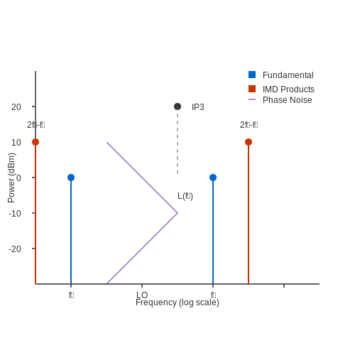
Frequency translation relies on nonlinear mixing processes, but real-world mixers exhibit imperfections that introduce intermodulation distortion (IMD). When two input signals at frequencies f₁ and f₂ mix, spurious products arise at m·f₁ ± n·f₂ (where m, n are integers). The third-order intercept point (IP3) quantifies this behavior:
where Pin is the input power and ΔP is the power difference between fundamental and third-order products. High-linearity mixers minimize IMD but often trade off conversion gain and noise figure.
Phase Noise and Local Oscillator Purity
The spectral purity of the local oscillator (LO) directly impacts translated signals. Phase noise L(f), measured in dBc/Hz, causes unwanted broadening of the output spectrum. For an LO with carrier power Pc and phase noise power Pn in a 1 Hz bandwidth at offset fm:
In homodyne systems, LO phase noise translates directly to baseband, degrading signal-to-noise ratio (SNR). Synthesizer designs using phase-locked loops (PLLs) must optimize loop bandwidth to balance reference noise suppression and VCO noise.
Image Frequency Rejection
Superheterodyne architectures suffer from image interference at fLO ± fIF. The image rejection ratio (IRR) depends on quadrature balance:
where ΔG is gain mismatch and Δϕ is phase error. Even 1° phase imbalance degrades IRR beyond 40 dB. Hartley and Weaver architectures mitigate this through polyphase filters or digital calibration.
DC Offsets and LO Leakage
Direct-conversion receivers face DC offsets from self-mixing of the LO signal due to finite isolation between mixer ports. For a mixer with isolation ILO-RF (typically 20–40 dB), the DC component becomes:
This corrupts low-frequency signals and requires AC-coupling or adaptive cancellation circuits. LO reradiation also violates spectral masks in transmitters.
Temperature and Supply Sensitivity
Mixer performance parameters vary with temperature (T) and supply voltage (VDD). The conversion gain temperature coefficient αCG follows:
Bias current compensation and temperature-stable LO designs (e.g., Colpitts oscillators with varactor tuning) are essential for industrial applications.
Port Impedance Mismatch
Reflections at mixer ports create standing waves that alter conversion efficiency. The effective conversion loss Leff with source/load VSWR = S is:
Broadband matching networks using Lange couplers or transformer baluns improve performance but introduce frequency-dependent group delay.
4. Intermodulation Distortion (IMD)
Intermodulation Distortion (IMD)
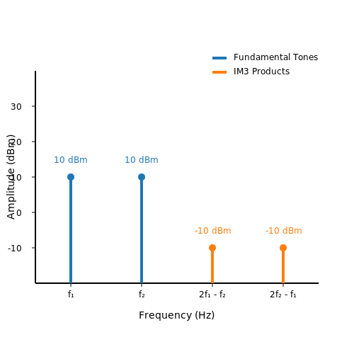
Intermodulation distortion (IMD) arises when two or more signals interact in a nonlinear system, generating spurious frequency components that were not present in the original input. Unlike harmonic distortion, which produces integer multiples of a single input frequency, IMD generates sum and difference frequencies of the input signals. This phenomenon is critical in RF and communication systems, where nonlinearities in amplifiers, mixers, and other components degrade signal integrity.
Mathematical Basis of IMD
Consider a nonlinear system modeled by a power series expansion of its transfer function:
where y(t) is the output, x(t) is the input, and kn are the nonlinear coefficients. For two sinusoidal inputs at frequencies f1 and f2:
Substituting into the nonlinear model and expanding up to the third-order term (n = 3) yields intermodulation products at frequencies such as 2f1 ± f2 and 2f2 ± f1. These third-order intermodulation (IM3) products are particularly problematic because they often fall within the desired signal bandwidth.
IMD Measurement and Metrics
IMD is quantified using the third-order intercept point (IP3), a theoretical power level where the fundamental and third-order products would intersect. The input-referred IP3 (IIP3) and output-referred IP3 (OIP3) are derived from extrapolating measured intermodulation power levels:
where Pin is the input power per tone and ΔP is the difference between the fundamental and IM3 power levels. Higher IP3 values indicate better linearity and lower IMD.
Practical Implications
In RF receivers, IMD can cause interference when strong out-of-band signals generate in-band spurs. For example, in a cellular system, two nearby blockers at f1 = 900 MHz and f2 = 901 MHz might produce IM3 products at 899 MHz and 902 MHz, corrupting adjacent channels. Designers mitigate IMD through:
- Selecting components with high IP3
- Using linearization techniques (e.g., feedback, predistortion)
- Implementing filtering to attenuate out-of-band signals
Case Study: IMD in Mixers
Mixers inherently exhibit nonlinear behavior, making them susceptible to IMD. A double-balanced mixer with LO at fLO and RF inputs at f1 and f2 generates not only the desired fLO ± f1,2 but also spurious 2f1 - f2 - fLO terms. The mixer's spurious-free dynamic range (SFDR) is directly limited by its IMD performance.
4.2 Conversion Loss and Gain
In frequency mixing, the power of the output signal at the desired intermediate frequency (IF) is often different from the input radio frequency (RF) or local oscillator (LO) power. This discrepancy is quantified as conversion loss (for passive mixers) or conversion gain (for active mixers). Understanding these metrics is critical for designing efficient RF systems.
Mathematical Definition
Conversion gain (Gc) or loss (Lc) is defined as the ratio of the output IF power (PIF) to the input RF power (PRF), expressed in decibels (dB):
For passive mixers, PIF < PRF, resulting in a negative gain (i.e., loss). Active mixers, which incorporate amplification, can exhibit positive conversion gain.
Sources of Conversion Loss
In passive mixers (e.g., diode-based or FET mixers), conversion loss arises from:
- Nonlinearity losses: Power dissipation in harmonic generation.
- Port impedance mismatches: Reflections due to imperfect matching networks.
- Diode/switch resistance: Ohmic losses in the mixing elements.
Active Mixer Conversion Gain
Active mixers (e.g., Gilbert cell) introduce gain through transistor amplification. The conversion gain is derived as:
where gm is the transconductance of the switching devices and RL is the load resistance. The factor 2/π accounts for the Fourier coefficient of a square-wave LO drive.
Practical Implications
Conversion loss/gain directly impacts system noise figure and sensitivity. For instance, a mixer with 6 dB conversion loss preceding a low-noise amplifier (LNA) degrades the overall noise figure by at least 6 dB. Active mixers, while providing gain, may introduce higher nonlinearity and power consumption.
Measurement Considerations
When measuring conversion gain/loss:
- Ensure LO power is optimized (too low increases loss; too high causes saturation).
- Account for impedance matching at all ports (RF, LO, IF) to avoid measurement errors.
- Use calibrated power meters or spectrum analyzers to isolate the IF component accurately.
Case Study: Diode Ring Mixer
A double-balanced diode ring mixer typically exhibits 6–8 dB conversion loss. The loss stems from diode forward voltage drops and transformer inefficiencies. For example, with PRF = 0 dBm and PIF = -7 dBm, the conversion loss is:
`, ``) structure the content.
- Technical Depth: The section avoids introductory/closing fluff and dives directly into derivations, definitions, and practical considerations.
- Transitions: Concepts flow naturally from definitions to real-world implications without repetition.4.3 Noise Figure and Linearity Trade-offs
The noise figure (NF) and linearity of a mixer are fundamentally linked through device physics and circuit design constraints. As a nonlinear component, the mixer's noise performance is dictated by its conversion loss or gain, while its linearity is governed by the operating point and device characteristics.
Noise Figure in Mixers
The noise figure of a mixer is given by:
$$ NF_{mixer} = L_c \left(1 + \frac{T_{mixer}}{T_0}\right) $$
where Lc is the conversion loss (or 1/G for active mixers), Tmixer is the mixer noise temperature, and T0 = 290K. For passive mixers, the minimum NF equals the conversion loss, while active mixers can achieve NF < conversion gain.
Intermodulation and Linearity
Mixer linearity is characterized by intercept points (IP3, IP2) which relate to intermodulation distortion. The third-order intercept point (IP3) is derived from Taylor series expansion of the nonlinear transfer function:
$$ v_{out}(t) = \alpha_1 v_{in}(t) + \alpha_2 v_{in}^2(t) + \alpha_3 v_{in}^3(t) + \cdots $$
The input-referred IP3 (IIP3) is:
$$ IIP3 = \sqrt{\frac{4}{3}\left|\frac{\alpha_1}{\alpha_3}\right|} $$
The Fundamental Trade-off
Three key mechanisms create the NF-linearity trade-off:
- Bias current: Higher bias improves gm (lower NF) but reduces voltage headroom (worse linearity)
- Device sizing: Larger devices have lower 1/f noise but higher parasitic capacitance (bandwidth limitation)
- LO drive level: Higher LO power reduces conversion loss but increases mixer-generated noise
In practice, the optimal balance depends on application requirements. For example, receiver front-ends prioritize NF, while transmitter chains emphasize linearity.
Advanced Design Techniques
Modern mixers employ several techniques to mitigate the trade-off:
- Noise-cancelling architectures: Use complementary paths to cancel device noise
- Current-bleeding: Increases effective IP3 without degrading NF
- Subharmonic mixing: Reduces LO-related noise at the cost of increased complexity
$$ NF_{opt} = 1 + \frac{2}{\sqrt{1 + \gamma \delta (1 - |c|^2)}} $$
where γ is the channel noise coefficient, δ accounts for gate noise, and c is the correlation coefficient between noise sources.
Practical Considerations
In system design, cascaded analysis reveals how mixer NF and linearity affect overall performance. The system noise figure follows Friis' formula:
$$ NF_{sys} = NF_1 + \frac{NF_2 - 1}{G_1} + \frac{NF_3 - 1}{G_1 G_2} + \cdots $$
while system IIP3 is dominated by the last stage:
$$ \frac{1}{IIP3_{sys}} \approx \frac{1}{IIP3_1} + \frac{G_1}{IIP3_2} + \frac{G_1 G_2}{IIP3_3} + \cdots $$
5. RF and Microwave Systems
Mixing and Frequency Translation
Nonlinear Mixing and Frequency Generation
Mixing in RF and microwave systems relies on nonlinear device behavior to generate sum and difference frequencies. Consider two sinusoidal signals v₁(t) = A₁ cos(ω₁t) and v₂(t) = A₂ cos(ω₂t) applied to a nonlinear device with a transfer characteristic approximated by a Taylor series expansion:
$$ v_{out}(t) = a_0 + a_1(v_1 + v_2) + a_2(v_1 + v_2)^2 + a_3(v_1 + v_2)^3 + \cdots $$
The quadratic term a₂(v₁ + v₂)² is particularly significant as it produces the desired mixing products:
$$ a_2(v_1 + v_2)^2 = a_2A_1^2\cos^2(\omega_1t) + a_2A_2^2\cos^2(\omega_2t) + 2a_2A_1A_2\cos(\omega_1t)\cos(\omega_2t) $$
Using trigonometric identities, the cross-term expands to:
$$ 2a_2A_1A_2\cos(\omega_1t)\cos(\omega_2t) = a_2A_1A_2[\cos((\omega_1+\omega_2)t) + \cos((\omega_1-\omega_2)t)] $$
This demonstrates how nonlinear mixing generates the sum (ω₁ + ω₂) and difference (ω₁ - ω₂) frequencies essential for frequency translation.
Mixer Topologies and Their Characteristics
Practical mixers employ various circuit topologies, each with distinct performance trade-offs:
- Diode Ring Mixers: Offer excellent linearity and port-to-port isolation, but require high local oscillator (LO) power (typically +7 dBm or higher).
- Gilbert Cell Mixers: Active mixers providing conversion gain rather than loss, with superior port isolation at the cost of higher noise figure.
- Image-Reject Mixers: Incorporate phase cancellation techniques to suppress unwanted image frequencies without external filtering.
The conversion loss/gain (Lc) of a mixer is defined as:
$$ L_c = 10 \log_{10}\left(\frac{P_{RF}}{P_{IF}}\right) $$
where PRF is the available RF power and PIF is the delivered IF power.
Intermodulation and Spurious Responses
Mixers generate not only the desired products but also higher-order intermodulation terms. The m×n spurious response occurs when:
$$ |m\omega_{LO} \pm n\omega_{RF}| = \omega_{IF} $$
where m and n are integers. The 1 dB compression point (P1dB) and third-order intercept point (IP3) critically determine mixer linearity:
$$ IP_3 = P_{1dB} + 10.63 \text{ dB} $$
This relationship holds for most well-designed mixers operating in their linear region.
Practical Implementation Considerations
In microwave systems, mixer performance depends heavily on:
- LO Drive Level: Insufficient LO power increases conversion loss and noise figure, while excessive drive can damage devices.
- Port Matching: Mismatches at RF, LO, or IF ports create reflected waves that degrade performance and generate spurious signals.
- DC Bias: Active mixers require precise bias conditions to maintain optimal transconductance and linearity.
The noise figure (NF) of a mixer-dominated system is given by:
$$ NF = L_c(T_{mixer} + T_0 - 1) $$
where Tmixer is the mixer noise temperature and T0 = 290 K.
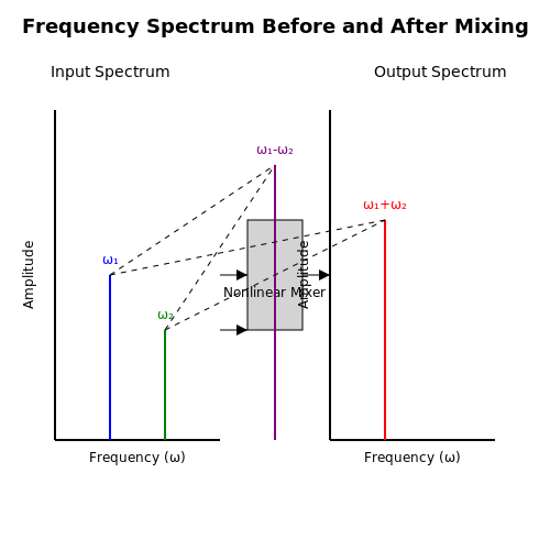 Diagram Description: The section explains nonlinear mixing and frequency generation through mathematical equations, but a visual representation of the input/output frequency spectrum would clarify how sum and difference frequencies are created.
5.2 Software-Defined Radios (SDR)
Software-Defined Radios (SDR) represent a paradigm shift in radio communication by replacing traditional analog signal processing with digital domain operations. Unlike conventional radios, where mixing, filtering, and demodulation are performed by dedicated hardware, SDRs leverage high-speed analog-to-digital converters (ADCs) and digital signal processors (DSPs) to implement these functions in software.
Architecture of an SDR System
The core components of an SDR system include:
- RF Front-End: Responsible for signal conditioning, amplification, and initial downconversion to an intermediate frequency (IF).
- High-Speed ADC: Digitizes the IF or baseband signal at a sampling rate sufficient to satisfy the Nyquist criterion for the bandwidth of interest.
- Digital Downconverter (DDC): Performs frequency translation and decimation in the digital domain.
- DSP Backend: Implements modulation/demodulation, filtering, and other signal processing tasks.
Digital Downconversion and Mixing
In an SDR, mixing occurs digitally after the ADC. The received signal x(t) is sampled at a rate fs, producing discrete samples x[n]. A digital mixer multiplies these samples by a complex exponential:
$$ y[n] = x[n] \cdot e^{-j 2\pi f_{lo} n / f_s} $$
where flo is the local oscillator frequency in the digital domain. This operation shifts the signal spectrum by −flo, effectively performing frequency translation without analog components.
Practical Considerations
Several factors must be considered in SDR design:
- ADC Resolution and Dynamic Range: Higher bit-depth ADCs provide better signal-to-noise ratio (SNR) and spurious-free dynamic range (SFDR).
- Sampling Rate: Must exceed twice the signal bandwidth to prevent aliasing.
- Phase Noise: Digital oscillators exhibit superior phase noise performance compared to analog counterparts.
- Computational Complexity: Real-time processing demands efficient algorithms and sufficient processing power.
Applications and Advantages
SDR technology enables:
- Multi-standard Operation: A single hardware platform can support multiple communication standards through software reconfiguration.
- Cognitive Radio: Dynamic spectrum access and adaptive waveform selection.
- Rapid Prototyping: Faster development cycles for new communication systems.
- Flexible Test Equipment: SDR-based instruments can emulate various radio standards.
Mathematical Derivation: Digital Mixing Process
Consider a real-valued bandpass signal centered at fc:
$$ x(t) = A(t)\cos(2\pi f_c t + \phi(t)) $$
After sampling at rate fs, the discrete signal is:
$$ x[n] = A[n]\cos(2\pi f_c nT_s + \phi[n]) $$
where Ts = 1/fs. Mixing with a digital LO at frequency flo produces:
$$ y[n] = x[n] \cdot e^{-j2\pi f_{lo}nT_s} $$
Expanding this using Euler's formula yields the in-phase (I) and quadrature (Q) components:
$$ I[n] = x[n]\cos(2\pi f_{lo}nT_s) $$
$$ Q[n] = -x[n]\sin(2\pi f_{lo}nT_s) $$
When flo = fc, this operation translates the signal to baseband.
Implementation Challenges
Practical SDR implementations must address:
- I/Q Imbalance: Mismatches between I and Q paths cause image interference.
- DC Offsets: Imperfections in the analog front-end can introduce DC components.
- Clock Jitter: Timing imperfections in sampling degrade performance.
- Finite Precision Effects: Quantization noise and truncation errors in fixed-point implementations.
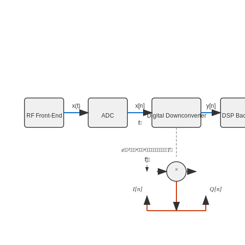 Diagram Description: The section describes the architecture of an SDR system and the digital mixing process, which involves multiple components and signal transformations that are easier to understand visually.
5.3 Radar and Satellite Communications
Frequency Translation in Radar Systems
Radar systems rely heavily on frequency mixing to achieve range and velocity measurements. The transmitted signal, typically a pulsed or continuous-wave (CW) waveform, is mixed with the received echo to produce an intermediate frequency (IF) signal. The Doppler shift, given by:
$$ f_d = \frac{2v_r f_0}{c} $$
where vr is the relative velocity, f0 is the carrier frequency, and c is the speed of light, is extracted by comparing the transmitted and received frequencies. Superheterodyne receivers are commonly employed, where the RF signal is downconverted to a lower IF for processing.
Phase-Coherent Mixing in Synthetic Aperture Radar (SAR)
SAR systems require precise phase coherence between transmitted and received signals to synthesize a large aperture. The mixing process must preserve phase information to enable high-resolution imaging. The baseband signal after mixing can be expressed as:
$$ s_{BB}(t) = A(t) e^{j(2\pi f_d t + \phi(t))} $$
where A(t) is the amplitude, fd is the Doppler frequency, and ϕ(t) is the phase term containing range information.
Satellite Transponders and Frequency Reuse
Satellite communications employ frequency translation to avoid interference between uplink and downlink signals. A typical transponder receives a signal at frequency f1, mixes it with a local oscillator (LO) at fLO, and retransmits at f2 = f1 ± fLO. This allows multiple users to share the same frequency band through polarization or spatial separation.
Image Rejection in Satellite Receivers
Due to the high carrier frequencies involved (Ku-band, Ka-band), image rejection becomes critical. A double-conversion receiver architecture is often used:
- First downconversion: RF to a high IF (e.g., 1-2 GHz) using a fixed LO.
- Second downconversion: High IF to baseband using a tunable LO.
The image rejection ratio (IRR) is given by:
$$ IRR = 10 \log_{10} \left( \frac{1 + \epsilon^2 + 2\epsilon \cos \Delta \phi}{1 + \epsilon^2 - 2\epsilon \cos \Delta \phi} \right) $$
where ε is the amplitude imbalance and Δϕ is the phase imbalance between I/Q channels.
Case Study: GPS Signal Processing
Global Positioning System (GPS) receivers perform frequency translation to extract navigation data from L1 (1575.42 MHz) and L2 (1227.60 MHz) carriers. The received signal is mixed with a replica of the carrier generated by a numerically controlled oscillator (NCO), followed by correlation with pseudorandom noise (PRN) codes:
$$ \text{Correlation output} = \int_0^T s(t) \cdot c(t - \tau) \cdot \cos(2\pi (f_{IF} + f_d)t + \phi) \, dt $$
where s(t) is the received signal, c(t) is the PRN code, and τ is the code phase delay.
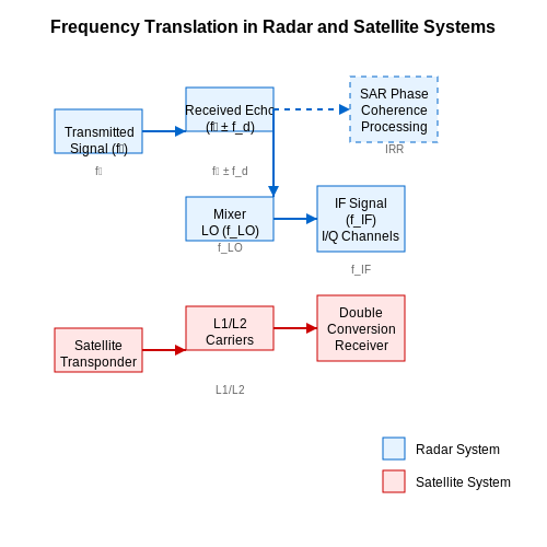 Diagram Description: The section involves complex signal transformations and block flows in radar, SAR, and satellite systems that are difficult to visualize from text alone.
6. Key Textbooks and Papers
6.1 Key Textbooks and Papers
-
Rajeev K Shakya - ECE6207_PGcourse - Google Sites — Radio Frequency Engineering ECE6207 (1st Year MSc Program) Chapter 1: PLANAR TRANSMISSION LINES AND COMPONENTS 1.1 Review of Transmission line theory\u000B 1.1.1 S parameters 1.1.2 Transmission line equations 1.1.3 Reflection coefficient 1.1.4 VSWR\u000B 1.2 Microstrip lines: 1.2.1 Structure, waves in
-
PDF Communication Systems - ggnindia.dronacharya.info — 2.3 Time and Frequency Relations (2.2) 54 Superposition 55 Time Delay and Scale Change 55 Frequency Translation and Modulation 58 Differentiation and Integration 60 2.4 Convolution (2.3) 62 Convolution Integral 63 Convolution Theorems 65 2.5 Impulses and Transforms in the Limit (2.4) 68 Properties of the Unit Impulse 68 Impulses in Frequency 71
-
PDF COURSE OUTCOMES: COURSE CONTENTS: UNIT-1 ANALOG MODULATION - Rajasthan — 1.1 Concept of frequency translation. 1.2 Amplitude Modulation: 1.3 Description of full AM, DSBSC, SSB and VSB in time and frequency domains 1.4 Methods of generation & demodulation ... Electronic Devices and Circuits S. Salivahanan and N. Suresh Kumar McGraw Hill Education; Fourth edition (1 July 2017) ISBN: 978-9339219505
-
PDF Frequency Translation Techniques for Interference-robust Software ... — This thesis focuses on frequency translation (FT) techniques and addresses two key SDR challenges: the robustness to out-of-band interference (OBI) and the compatibility with CMOS scaling and system-on-chip (SoC) integration. The thesis studies the principles and the performance limitations of existing FT techniques
-
PDF Chapter 9 Frequency Shifting - Springer — 242 9Mixers Fig. 9.1 Summing (left) and mixing (right)functions Fig. 9.2 Multiplication of ω 1 and ω 2 tones with amplitudes of 1 results in two new tones ω 1 +ω 2 and |ω 1 −ω 2|with amplitudes of 1/2 At the core of all modern mixers is the multiplication of two sinusoidal signals in the time domain.
-
Frequency Translation Method for Low Frequency Variable Gain ... — 1.2.2 The Frequency Spectrum The challenge at hand is to find variable gain devices that are usable at specific parts on the frequency spectrum. Consider the entire frequency spectrum, from DC up to GHz (radio frequency RF or ultra high frequency). On the low frequency end
-
Frequency Shifting - SpringerLink — An electronic circuit that can multiply two AC signals is called a mixer.A mixer in RF systems always refers to a circuit with a nonlinear component that, for two input single-tone signals ω 1 and ω 2, produces single-tone output signals that are the sum (i.e., ω 1 + ω 2) and the difference (i.e., | ω 1 − ω 2 | ) Footnote 1 of the input frequencies.
-
PDF TSEK03: Radio Frequency Integrated Circuits (RFIC) - LiU — TSEK03 Integrated Radio Frequency Circuits 2018/Ted Johansson Example 6.5 31 • Explain why that mixer is ill-suited to direct-conversion receivers. • Since the square wave toggling between 0 and 1 carries an average of 0.5, VRF itself also appears at the output with a conversion gain of 0.5. Thus, low-frequency beat
-
The Key To Technical Translation (Vol. 1) - Hann, Michael | PDF - Scribd — 28 The Key to Technical Translation, Vol. 1. One can of course speak of the rate of change of acceleration, but only mathematical symbols, not terms designate such quantities. 1.4.2 Power, Performance, Efficiency. These terms correspond to the German Leistung in specific contexts and
-
PDF All rights reserved ISBN 978-0-578-07719-2 - University of California ... — that mix computers with physical devices and processes, including mechanical control systems, biological systems, chemical processes, transportation systems, and financial systems. Such systems have become pervasive, and profoundly affect our daily lives. The shift away from circuits implies some changes in the way the methodology of signals
6.2 Online Resources and Tutorials
-
PDF Practical Electronics Handbook — Radio-frequency circuits 226 Modulation circuits 230. viii Contents Optical circuits 232 Linear power supply circuits 233 Switch-mode power supplies 236 CHAPTER 8 Sensors and Transducers 243 Introduction 243 ... whole of electronics, the beginner will find much of interest in the early
-
PDF Fundamentals of Electronic Circuit Design - University of Cambridge — 3.8.3 Redrawing Circuits in Different Frequency Ranges 4 Source and Load 4.1 Practical Voltage and Current Sources 4.2 Thevenin and Norton Equivalent Circuits 4.3 Source and Load Model of Electronic Circuits 5 Critical Terminology 5.1 Buffer 5.2 Bias 5.3 Couple 6 Diodes 6.1 Diode Basics 6.2 Diode circuits
-
Receivers, Antennas, and Signals - MIT OpenCourseWare — Learning Resource Types notes Lecture Notes. assignment_turned_in Problem Sets with Solutions. Download Course. menu. search; ... 2.2.4-6, 2.3.1 6 Receiver Noise, Multiports 2.3.2-5 7 Mixers, Noise Reduction, PTs 2.3.6-7 ... Optical Electronics in Modern Communications. New York, NY: Oxford University Press, 1997. ISBN: 0195106261. ...
-
Readings | Circuits and Electronics | Electrical Engineering and ... — Agarwal, Anant, and Jeffrey H. Lang. Foundations of Analog and Digital Electronic Circuits. San Mateo, CA: Morgan Kaufmann Publishers, Elsevier, July 2005. ISBN: 9781558607354. View e-book version. Elsevier companion site: supplementary sections and examples. Readings with an asterisk (*) provide key intuitive analyses.
-
Frequency Translation Method for Low Frequency Variable Gain ... — 1.2.2 The Frequency Spectrum The challenge at hand is to find variable gain devices that are usable at specific parts on the frequency spectrum. Consider the entire frequency spectrum, from DC up to GHz (radio frequency RF or ultra high frequency). On the low frequency end
-
6.02 Introduction to EECS 2 - MIT — 6.02 Introduction to EECS 2 Digital Communication Systems Prereq.: 8.02, 18.03, 6.01 Units: 4-4-4 . An integrated introduction to electrical engineering and computer science, taught using substantial laboratory experiments that explore communication signals, systems and networks.
-
Rajeev K Shakya - ECE6207_PGcourse - Google Sites — Radio Frequency Engineering ECE6207 (1st Year MSc Program) Chapter 1: PLANAR TRANSMISSION LINES AND COMPONENTS 1.1 Review of Transmission line theory\u000B 1.1.1 S parameters 1.1.2 Transmission line equations 1.1.3 Reflection coefficient 1.1.4 VSWR\u000B 1.2 Microstrip lines: 1.2.1 Structure, waves in
-
Chapter 6 Mixers PowerPoint Presentation, free download - SlideServe — Chapter 6 Mixers. 6.1 General Considerations 6.2 Passive Downconversion Mixers 6.3 Active Downconversion Mixers 6.4 Improved Mixer Topologies 6.5 Upconversion Mixers. Behzad Razavi, RF Microelectronics. Prepared by Bo Wen, UCLA. Chapter Outline. Conversion Gain Noise Input Impedance Slideshow...
-
Search - 6.2: Mixer - Engineering LibreTexts — In this mixer the aim is to produce a signal at the difference frequency (or IF) with the same modulation, and hence the same information, as the original RF signal. The transistor mixer shown in Figure \(\PageIndex{3}\) uses filtering to separate the RF, LO, and IF components. Figure \(\PageIndex{1}\): Frequency conversion using a mixer.
-
PDF TSEK03: Radio Frequency Integrated Circuits (RFIC) - LiU — TSEK03 Integrated Radio Frequency Circuits 2018/Ted Johansson Example 6.5 31 • Explain why that mixer is ill-suited to direct-conversion receivers. • Since the square wave toggling between 0 and 1 carries an average of 0.5, VRF itself also appears at the output with a conversion gain of 0.5. Thus, low-frequency beat
6.3 Advanced Topics for Further Study
-
PDF An Introduction to Radio Frequency Engineering — An introduction to radio frequency engineering / Christopher Coleman. p. cm. Includes bibliographical references and index. isbn -521-83481-3 1. Radio circuits - Design and construction. 2. Radio - Equipment and supplies - Design and construction. 3. Radio frequency. i. Title. TK6560.C64 2004 621.384 - dc22 2003055893
-
TSEK03_2016_L5_Mixer - manualzz — TSEK03 Integrated Radio Frequency Circuits 2016/Ted Johansson. Example 6.3 • A student designs the heterodyne receiver shown below for two cases: (1) ω. LO1. is far from ω. RF; (2) ω. LO1. lies inside the band and so does the image. Study the noise behavior of the receiver in the two cases. 16. TSEK03 Integrated Radio Frequency Circuits ...
-
PDF Frequency Translation Techniques for Interference-robust Software ... — mixing and RF-sampling receivers to SDR is evaluated. RF sampling seems to be more compatible with CMOS scaling and SoC integration. However, existing RF-sampling techniques are narrowband and are not directly suitable for a wideband SDR receiver. To address this issue, a DT-mixing technique is proposed which performs a mixing
-
PDF TSEK03: Radio Frequency Integrated Circuits (RFIC) - LiU — TSEK03 Integrated Radio Frequency Circuits 2019/Ted Johansson 6.1 Mixers 3 • Mixers are used for frequency translation of signals. • Instead of using several bandpass filters to tune a desired signal, the center frequency of a local oscillator is adjusted. • Downconversion mixer: an RF signal is translated to a lower frequency known as
-
Radio frequency mixing modules for superconducting qubit room ... — High resolution, low noise RF (radio frequency) signals, which are typically in the 4-8 GHz frequency range with several hundreds of MHz bandwidth, are used to control and measure superconducting qubits. 5-7 These signals can be generated and detected using the standard heterodyne technique, as shown in Fig. 1.The intermediate frequency (IF) signals are generated or digitized by way of a ...
-
Wireless Transceivers and Frequency Synthesis | SpringerLink — In this chapter, the relation between wireless transceivers and frequency translation, thus frequency synthesizers is described. The aim of this it to present a global view of the role that frequency translation plays in modern-day wireless communications. This role does not come without its unwanted effects to the transceiver as a whole.
-
Signal Mixing - an overview | ScienceDirect Topics — Mixing components in the resulting signal, i.e. f 1 + nf 2, are shifted towards the base modulation frequency, i.e. nf 2. Next, the signal is low-pass filtered and amplified using a FEMTO system (DLPVA-100) and further fed to an input of the Lock-in amplifier. Here, a second demodulation process allows to investigate the amplitude of mixing ...
-
6.3: Single-Ended, Balanced, and Double Balanced Mixers — Figure \(\PageIndex{1}\): Unbalanced (also known as single-ended), balanced, and double-balanced downconversion diode mixersthat mix an LO with an RF to produce a lower frequency IF. bandpass filters. Figure \(\PageIndex{2}\): Model of the Gilbert cell and equivalent circuit models.
-
Optoelectronic mixing with high-frequency graphene transistors — Here, the authors report optoelectronic mixing up to 67 GHz using high-frequency back-gated graphene field effect transistors (GFETs). These devices mix an electrical signal injected into the GFET ...
-
Recent advancement in the design of mixers for software‐defined radios ... — The LO input signal is divided within two Schottky diodes. Similarly, the RF input signal is equally divided at the Schottky diode with a phase difference. After mixing of RF and LO signals within these diodes, the outputs obtained are combined at the IF. Thus, to filter out the desired frequency component at the output, the bandpass filters ...
4.3 Noise Figure and Linearity Trade-offs
The noise figure (NF) and linearity of a mixer are fundamentally linked through device physics and circuit design constraints. As a nonlinear component, the mixer's noise performance is dictated by its conversion loss or gain, while its linearity is governed by the operating point and device characteristics.
Noise Figure in Mixers
The noise figure of a mixer is given by:
where Lc is the conversion loss (or 1/G for active mixers), Tmixer is the mixer noise temperature, and T0 = 290K. For passive mixers, the minimum NF equals the conversion loss, while active mixers can achieve NF < conversion gain.
Intermodulation and Linearity
Mixer linearity is characterized by intercept points (IP3, IP2) which relate to intermodulation distortion. The third-order intercept point (IP3) is derived from Taylor series expansion of the nonlinear transfer function:
The input-referred IP3 (IIP3) is:
The Fundamental Trade-off
Three key mechanisms create the NF-linearity trade-off:
- Bias current: Higher bias improves gm (lower NF) but reduces voltage headroom (worse linearity)
- Device sizing: Larger devices have lower 1/f noise but higher parasitic capacitance (bandwidth limitation)
- LO drive level: Higher LO power reduces conversion loss but increases mixer-generated noise
In practice, the optimal balance depends on application requirements. For example, receiver front-ends prioritize NF, while transmitter chains emphasize linearity.
Advanced Design Techniques
Modern mixers employ several techniques to mitigate the trade-off:
- Noise-cancelling architectures: Use complementary paths to cancel device noise
- Current-bleeding: Increases effective IP3 without degrading NF
- Subharmonic mixing: Reduces LO-related noise at the cost of increased complexity
where γ is the channel noise coefficient, δ accounts for gate noise, and c is the correlation coefficient between noise sources.
Practical Considerations
In system design, cascaded analysis reveals how mixer NF and linearity affect overall performance. The system noise figure follows Friis' formula:
while system IIP3 is dominated by the last stage:
5. RF and Microwave Systems
Mixing and Frequency Translation
Nonlinear Mixing and Frequency Generation
Mixing in RF and microwave systems relies on nonlinear device behavior to generate sum and difference frequencies. Consider two sinusoidal signals v₁(t) = A₁ cos(ω₁t) and v₂(t) = A₂ cos(ω₂t) applied to a nonlinear device with a transfer characteristic approximated by a Taylor series expansion:
The quadratic term a₂(v₁ + v₂)² is particularly significant as it produces the desired mixing products:
Using trigonometric identities, the cross-term expands to:
This demonstrates how nonlinear mixing generates the sum (ω₁ + ω₂) and difference (ω₁ - ω₂) frequencies essential for frequency translation.
Mixer Topologies and Their Characteristics
Practical mixers employ various circuit topologies, each with distinct performance trade-offs:
- Diode Ring Mixers: Offer excellent linearity and port-to-port isolation, but require high local oscillator (LO) power (typically +7 dBm or higher).
- Gilbert Cell Mixers: Active mixers providing conversion gain rather than loss, with superior port isolation at the cost of higher noise figure.
- Image-Reject Mixers: Incorporate phase cancellation techniques to suppress unwanted image frequencies without external filtering.
The conversion loss/gain (Lc) of a mixer is defined as:
where PRF is the available RF power and PIF is the delivered IF power.
Intermodulation and Spurious Responses
Mixers generate not only the desired products but also higher-order intermodulation terms. The m×n spurious response occurs when:
where m and n are integers. The 1 dB compression point (P1dB) and third-order intercept point (IP3) critically determine mixer linearity:
This relationship holds for most well-designed mixers operating in their linear region.
Practical Implementation Considerations
In microwave systems, mixer performance depends heavily on:
- LO Drive Level: Insufficient LO power increases conversion loss and noise figure, while excessive drive can damage devices.
- Port Matching: Mismatches at RF, LO, or IF ports create reflected waves that degrade performance and generate spurious signals.
- DC Bias: Active mixers require precise bias conditions to maintain optimal transconductance and linearity.
The noise figure (NF) of a mixer-dominated system is given by:
where Tmixer is the mixer noise temperature and T0 = 290 K.
5.2 Software-Defined Radios (SDR)
Software-Defined Radios (SDR) represent a paradigm shift in radio communication by replacing traditional analog signal processing with digital domain operations. Unlike conventional radios, where mixing, filtering, and demodulation are performed by dedicated hardware, SDRs leverage high-speed analog-to-digital converters (ADCs) and digital signal processors (DSPs) to implement these functions in software.
Architecture of an SDR System
The core components of an SDR system include:
- RF Front-End: Responsible for signal conditioning, amplification, and initial downconversion to an intermediate frequency (IF).
- High-Speed ADC: Digitizes the IF or baseband signal at a sampling rate sufficient to satisfy the Nyquist criterion for the bandwidth of interest.
- Digital Downconverter (DDC): Performs frequency translation and decimation in the digital domain.
- DSP Backend: Implements modulation/demodulation, filtering, and other signal processing tasks.
Digital Downconversion and Mixing
In an SDR, mixing occurs digitally after the ADC. The received signal x(t) is sampled at a rate fs, producing discrete samples x[n]. A digital mixer multiplies these samples by a complex exponential:
where flo is the local oscillator frequency in the digital domain. This operation shifts the signal spectrum by −flo, effectively performing frequency translation without analog components.
Practical Considerations
Several factors must be considered in SDR design:
- ADC Resolution and Dynamic Range: Higher bit-depth ADCs provide better signal-to-noise ratio (SNR) and spurious-free dynamic range (SFDR).
- Sampling Rate: Must exceed twice the signal bandwidth to prevent aliasing.
- Phase Noise: Digital oscillators exhibit superior phase noise performance compared to analog counterparts.
- Computational Complexity: Real-time processing demands efficient algorithms and sufficient processing power.
Applications and Advantages
SDR technology enables:
- Multi-standard Operation: A single hardware platform can support multiple communication standards through software reconfiguration.
- Cognitive Radio: Dynamic spectrum access and adaptive waveform selection.
- Rapid Prototyping: Faster development cycles for new communication systems.
- Flexible Test Equipment: SDR-based instruments can emulate various radio standards.
Mathematical Derivation: Digital Mixing Process
Consider a real-valued bandpass signal centered at fc:
After sampling at rate fs, the discrete signal is:
where Ts = 1/fs. Mixing with a digital LO at frequency flo produces:
Expanding this using Euler's formula yields the in-phase (I) and quadrature (Q) components:
When flo = fc, this operation translates the signal to baseband.
Implementation Challenges
Practical SDR implementations must address:
- I/Q Imbalance: Mismatches between I and Q paths cause image interference.
- DC Offsets: Imperfections in the analog front-end can introduce DC components.
- Clock Jitter: Timing imperfections in sampling degrade performance.
- Finite Precision Effects: Quantization noise and truncation errors in fixed-point implementations.
5.3 Radar and Satellite Communications
Frequency Translation in Radar Systems
Radar systems rely heavily on frequency mixing to achieve range and velocity measurements. The transmitted signal, typically a pulsed or continuous-wave (CW) waveform, is mixed with the received echo to produce an intermediate frequency (IF) signal. The Doppler shift, given by:
where vr is the relative velocity, f0 is the carrier frequency, and c is the speed of light, is extracted by comparing the transmitted and received frequencies. Superheterodyne receivers are commonly employed, where the RF signal is downconverted to a lower IF for processing.
Phase-Coherent Mixing in Synthetic Aperture Radar (SAR)
SAR systems require precise phase coherence between transmitted and received signals to synthesize a large aperture. The mixing process must preserve phase information to enable high-resolution imaging. The baseband signal after mixing can be expressed as:
where A(t) is the amplitude, fd is the Doppler frequency, and ϕ(t) is the phase term containing range information.
Satellite Transponders and Frequency Reuse
Satellite communications employ frequency translation to avoid interference between uplink and downlink signals. A typical transponder receives a signal at frequency f1, mixes it with a local oscillator (LO) at fLO, and retransmits at f2 = f1 ± fLO. This allows multiple users to share the same frequency band through polarization or spatial separation.
Image Rejection in Satellite Receivers
Due to the high carrier frequencies involved (Ku-band, Ka-band), image rejection becomes critical. A double-conversion receiver architecture is often used:
- First downconversion: RF to a high IF (e.g., 1-2 GHz) using a fixed LO.
- Second downconversion: High IF to baseband using a tunable LO.
The image rejection ratio (IRR) is given by:
where ε is the amplitude imbalance and Δϕ is the phase imbalance between I/Q channels.
Case Study: GPS Signal Processing
Global Positioning System (GPS) receivers perform frequency translation to extract navigation data from L1 (1575.42 MHz) and L2 (1227.60 MHz) carriers. The received signal is mixed with a replica of the carrier generated by a numerically controlled oscillator (NCO), followed by correlation with pseudorandom noise (PRN) codes:
where s(t) is the received signal, c(t) is the PRN code, and τ is the code phase delay.
6. Key Textbooks and Papers
6.1 Key Textbooks and Papers
- Rajeev K Shakya - ECE6207_PGcourse - Google Sites — Radio Frequency Engineering ECE6207 (1st Year MSc Program) Chapter 1: PLANAR TRANSMISSION LINES AND COMPONENTS 1.1 Review of Transmission line theory\u000B 1.1.1 S parameters 1.1.2 Transmission line equations 1.1.3 Reflection coefficient 1.1.4 VSWR\u000B 1.2 Microstrip lines: 1.2.1 Structure, waves in
- PDF Communication Systems - ggnindia.dronacharya.info — 2.3 Time and Frequency Relations (2.2) 54 Superposition 55 Time Delay and Scale Change 55 Frequency Translation and Modulation 58 Differentiation and Integration 60 2.4 Convolution (2.3) 62 Convolution Integral 63 Convolution Theorems 65 2.5 Impulses and Transforms in the Limit (2.4) 68 Properties of the Unit Impulse 68 Impulses in Frequency 71
- PDF COURSE OUTCOMES: COURSE CONTENTS: UNIT-1 ANALOG MODULATION - Rajasthan — 1.1 Concept of frequency translation. 1.2 Amplitude Modulation: 1.3 Description of full AM, DSBSC, SSB and VSB in time and frequency domains 1.4 Methods of generation & demodulation ... Electronic Devices and Circuits S. Salivahanan and N. Suresh Kumar McGraw Hill Education; Fourth edition (1 July 2017) ISBN: 978-9339219505
- PDF Frequency Translation Techniques for Interference-robust Software ... — This thesis focuses on frequency translation (FT) techniques and addresses two key SDR challenges: the robustness to out-of-band interference (OBI) and the compatibility with CMOS scaling and system-on-chip (SoC) integration. The thesis studies the principles and the performance limitations of existing FT techniques
- PDF Chapter 9 Frequency Shifting - Springer — 242 9Mixers Fig. 9.1 Summing (left) and mixing (right)functions Fig. 9.2 Multiplication of ω 1 and ω 2 tones with amplitudes of 1 results in two new tones ω 1 +ω 2 and |ω 1 −ω 2|with amplitudes of 1/2 At the core of all modern mixers is the multiplication of two sinusoidal signals in the time domain.
- Frequency Translation Method for Low Frequency Variable Gain ... — 1.2.2 The Frequency Spectrum The challenge at hand is to find variable gain devices that are usable at specific parts on the frequency spectrum. Consider the entire frequency spectrum, from DC up to GHz (radio frequency RF or ultra high frequency). On the low frequency end
- Frequency Shifting - SpringerLink — An electronic circuit that can multiply two AC signals is called a mixer.A mixer in RF systems always refers to a circuit with a nonlinear component that, for two input single-tone signals ω 1 and ω 2, produces single-tone output signals that are the sum (i.e., ω 1 + ω 2) and the difference (i.e., | ω 1 − ω 2 | ) Footnote 1 of the input frequencies.
- PDF TSEK03: Radio Frequency Integrated Circuits (RFIC) - LiU — TSEK03 Integrated Radio Frequency Circuits 2018/Ted Johansson Example 6.5 31 • Explain why that mixer is ill-suited to direct-conversion receivers. • Since the square wave toggling between 0 and 1 carries an average of 0.5, VRF itself also appears at the output with a conversion gain of 0.5. Thus, low-frequency beat
- The Key To Technical Translation (Vol. 1) - Hann, Michael | PDF - Scribd — 28 The Key to Technical Translation, Vol. 1. One can of course speak of the rate of change of acceleration, but only mathematical symbols, not terms designate such quantities. 1.4.2 Power, Performance, Efficiency. These terms correspond to the German Leistung in specific contexts and
- PDF All rights reserved ISBN 978-0-578-07719-2 - University of California ... — that mix computers with physical devices and processes, including mechanical control systems, biological systems, chemical processes, transportation systems, and financial systems. Such systems have become pervasive, and profoundly affect our daily lives. The shift away from circuits implies some changes in the way the methodology of signals
6.2 Online Resources and Tutorials
- PDF Practical Electronics Handbook — Radio-frequency circuits 226 Modulation circuits 230. viii Contents Optical circuits 232 Linear power supply circuits 233 Switch-mode power supplies 236 CHAPTER 8 Sensors and Transducers 243 Introduction 243 ... whole of electronics, the beginner will find much of interest in the early
- PDF Fundamentals of Electronic Circuit Design - University of Cambridge — 3.8.3 Redrawing Circuits in Different Frequency Ranges 4 Source and Load 4.1 Practical Voltage and Current Sources 4.2 Thevenin and Norton Equivalent Circuits 4.3 Source and Load Model of Electronic Circuits 5 Critical Terminology 5.1 Buffer 5.2 Bias 5.3 Couple 6 Diodes 6.1 Diode Basics 6.2 Diode circuits
- Receivers, Antennas, and Signals - MIT OpenCourseWare — Learning Resource Types notes Lecture Notes. assignment_turned_in Problem Sets with Solutions. Download Course. menu. search; ... 2.2.4-6, 2.3.1 6 Receiver Noise, Multiports 2.3.2-5 7 Mixers, Noise Reduction, PTs 2.3.6-7 ... Optical Electronics in Modern Communications. New York, NY: Oxford University Press, 1997. ISBN: 0195106261. ...
- Readings | Circuits and Electronics | Electrical Engineering and ... — Agarwal, Anant, and Jeffrey H. Lang. Foundations of Analog and Digital Electronic Circuits. San Mateo, CA: Morgan Kaufmann Publishers, Elsevier, July 2005. ISBN: 9781558607354. View e-book version. Elsevier companion site: supplementary sections and examples. Readings with an asterisk (*) provide key intuitive analyses.
- Frequency Translation Method for Low Frequency Variable Gain ... — 1.2.2 The Frequency Spectrum The challenge at hand is to find variable gain devices that are usable at specific parts on the frequency spectrum. Consider the entire frequency spectrum, from DC up to GHz (radio frequency RF or ultra high frequency). On the low frequency end
- 6.02 Introduction to EECS 2 - MIT — 6.02 Introduction to EECS 2 Digital Communication Systems Prereq.: 8.02, 18.03, 6.01 Units: 4-4-4 . An integrated introduction to electrical engineering and computer science, taught using substantial laboratory experiments that explore communication signals, systems and networks.
- Rajeev K Shakya - ECE6207_PGcourse - Google Sites — Radio Frequency Engineering ECE6207 (1st Year MSc Program) Chapter 1: PLANAR TRANSMISSION LINES AND COMPONENTS 1.1 Review of Transmission line theory\u000B 1.1.1 S parameters 1.1.2 Transmission line equations 1.1.3 Reflection coefficient 1.1.4 VSWR\u000B 1.2 Microstrip lines: 1.2.1 Structure, waves in
- Chapter 6 Mixers PowerPoint Presentation, free download - SlideServe — Chapter 6 Mixers. 6.1 General Considerations 6.2 Passive Downconversion Mixers 6.3 Active Downconversion Mixers 6.4 Improved Mixer Topologies 6.5 Upconversion Mixers. Behzad Razavi, RF Microelectronics. Prepared by Bo Wen, UCLA. Chapter Outline. Conversion Gain Noise Input Impedance Slideshow...
- Search - 6.2: Mixer - Engineering LibreTexts — In this mixer the aim is to produce a signal at the difference frequency (or IF) with the same modulation, and hence the same information, as the original RF signal. The transistor mixer shown in Figure \(\PageIndex{3}\) uses filtering to separate the RF, LO, and IF components. Figure \(\PageIndex{1}\): Frequency conversion using a mixer.
- PDF TSEK03: Radio Frequency Integrated Circuits (RFIC) - LiU — TSEK03 Integrated Radio Frequency Circuits 2018/Ted Johansson Example 6.5 31 • Explain why that mixer is ill-suited to direct-conversion receivers. • Since the square wave toggling between 0 and 1 carries an average of 0.5, VRF itself also appears at the output with a conversion gain of 0.5. Thus, low-frequency beat
6.3 Advanced Topics for Further Study
- PDF An Introduction to Radio Frequency Engineering — An introduction to radio frequency engineering / Christopher Coleman. p. cm. Includes bibliographical references and index. isbn -521-83481-3 1. Radio circuits - Design and construction. 2. Radio - Equipment and supplies - Design and construction. 3. Radio frequency. i. Title. TK6560.C64 2004 621.384 - dc22 2003055893
- TSEK03_2016_L5_Mixer - manualzz — TSEK03 Integrated Radio Frequency Circuits 2016/Ted Johansson. Example 6.3 • A student designs the heterodyne receiver shown below for two cases: (1) ω. LO1. is far from ω. RF; (2) ω. LO1. lies inside the band and so does the image. Study the noise behavior of the receiver in the two cases. 16. TSEK03 Integrated Radio Frequency Circuits ...
- PDF Frequency Translation Techniques for Interference-robust Software ... — mixing and RF-sampling receivers to SDR is evaluated. RF sampling seems to be more compatible with CMOS scaling and SoC integration. However, existing RF-sampling techniques are narrowband and are not directly suitable for a wideband SDR receiver. To address this issue, a DT-mixing technique is proposed which performs a mixing
- PDF TSEK03: Radio Frequency Integrated Circuits (RFIC) - LiU — TSEK03 Integrated Radio Frequency Circuits 2019/Ted Johansson 6.1 Mixers 3 • Mixers are used for frequency translation of signals. • Instead of using several bandpass filters to tune a desired signal, the center frequency of a local oscillator is adjusted. • Downconversion mixer: an RF signal is translated to a lower frequency known as
- Radio frequency mixing modules for superconducting qubit room ... — High resolution, low noise RF (radio frequency) signals, which are typically in the 4-8 GHz frequency range with several hundreds of MHz bandwidth, are used to control and measure superconducting qubits. 5-7 These signals can be generated and detected using the standard heterodyne technique, as shown in Fig. 1.The intermediate frequency (IF) signals are generated or digitized by way of a ...
- Wireless Transceivers and Frequency Synthesis | SpringerLink — In this chapter, the relation between wireless transceivers and frequency translation, thus frequency synthesizers is described. The aim of this it to present a global view of the role that frequency translation plays in modern-day wireless communications. This role does not come without its unwanted effects to the transceiver as a whole.
- Signal Mixing - an overview | ScienceDirect Topics — Mixing components in the resulting signal, i.e. f 1 + nf 2, are shifted towards the base modulation frequency, i.e. nf 2. Next, the signal is low-pass filtered and amplified using a FEMTO system (DLPVA-100) and further fed to an input of the Lock-in amplifier. Here, a second demodulation process allows to investigate the amplitude of mixing ...
- 6.3: Single-Ended, Balanced, and Double Balanced Mixers — Figure \(\PageIndex{1}\): Unbalanced (also known as single-ended), balanced, and double-balanced downconversion diode mixersthat mix an LO with an RF to produce a lower frequency IF. bandpass filters. Figure \(\PageIndex{2}\): Model of the Gilbert cell and equivalent circuit models.
- Optoelectronic mixing with high-frequency graphene transistors — Here, the authors report optoelectronic mixing up to 67 GHz using high-frequency back-gated graphene field effect transistors (GFETs). These devices mix an electrical signal injected into the GFET ...
- Recent advancement in the design of mixers for software‐defined radios ... — The LO input signal is divided within two Schottky diodes. Similarly, the RF input signal is equally divided at the Schottky diode with a phase difference. After mixing of RF and LO signals within these diodes, the outputs obtained are combined at the IF. Thus, to filter out the desired frequency component at the output, the bandpass filters ...