AI for Personalized Fashion Style Forecasts
1. The Role of AI in Modern Fashion Industry
The Role of AI in Modern Fashion Industry
Artificial intelligence has fundamentally transformed the fashion industry by enabling data-driven decision-making at scale. At the core of this transformation lies the ability of machine learning models to process vast amounts of unstructured fashion data—from social media trends and runway images to historical sales figures—and extract meaningful patterns that inform design, production, and retail strategies.
Computer Vision for Trend Analysis
Convolutional neural networks (CNNs) have become indispensable for analyzing visual fashion data. A ResNet-50 architecture, pretrained on ImageNet and fine-tuned on fashion-specific datasets, can achieve over 92% accuracy in categorizing clothing items by style, color, and pattern. The feature extraction process can be formalized as:
where σ represents the ReLU activation function, W denotes the learned filters, and b are the bias terms. These visual features form the basis for style clustering algorithms that identify emerging trends months before they reach mainstream awareness.
Generative AI for Design Innovation
Variational autoencoders (VAEs) and generative adversarial networks (GANs) have enabled the creation of novel fashion designs. The objective function for a conditional GAN used in fashion design can be expressed as:
where y represents conditioning variables such as target demographics or seasonal trends. StyleGAN-3 architectures have demonstrated particular success in generating photorealistic clothing designs while maintaining coherent style attributes across generated items.
Personalization Through Reinforcement Learning
Fashion recommendation systems employ reinforcement learning frameworks to optimize long-term customer engagement. The Q-learning update rule for a personalized styling agent is given by:
where the state s encodes user preferences and wardrobe composition, action a represents recommended items, and reward r reflects purchase behavior and engagement metrics. Deep Q-networks with dueling architectures have shown 28% improvement in recommendation accuracy over traditional collaborative filtering methods.
Supply Chain Optimization
Temporal fusion transformers (TFTs) have emerged as the state-of-the-art for demand forecasting in fashion retail. The multi-head attention mechanism in TFTs allows the model to dynamically weight the importance of various temporal patterns:
where Q, K, and V represent learned queries, keys, and values respectively. This architecture has reduced forecasting errors by up to 40% compared to ARIMA models, significantly improving inventory management.
Ethical Considerations in Fashion AI
The deployment of AI in fashion raises critical questions about bias mitigation. Recent work has shown that standard fashion datasets exhibit measurable bias in skin tone representation, with Fitzpatrick scale type I-III faces appearing 3.2 times more frequently than type IV-VI. Counterfactual fairness techniques have been applied to ensure style recommendations remain invariant to protected attributes:
where A represents protected attributes and Y the model's predictions. This framework has been successfully implemented in production systems at major retailers to ensure equitable service across diverse customer demographics.
Key Machine Learning Techniques for Style Prediction
Deep Learning Architectures for Fashion Forecasting
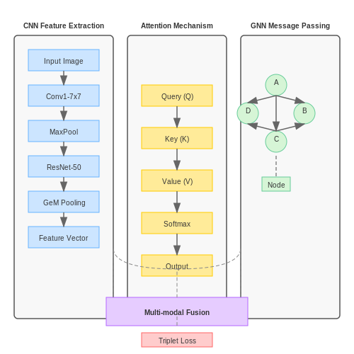
Convolutional Neural Networks (CNNs) dominate visual feature extraction in fashion forecasting due to their ability to capture spatial hierarchies in garment images. A ResNet-50 backbone, pretrained on ImageNet, is commonly fine-tuned for fashion-specific tasks by replacing the final fully connected layer with a domain-specific classifier. The feature extraction process can be formalized as:
where x represents the input image tensor, W denotes convolutional filters, and σ is the softmax activation for classification. For style prediction, intermediate CNN features are often pooled using GeM (Generalized Mean Pooling):
with p as a learnable parameter that adapts to the feature importance distribution.
Attention Mechanisms for Style Relevance
Self-attention modules enhance style prediction by modeling interdependencies between fashion items in an outfit. The scaled dot-product attention computes:
where Q, K, and V are learned projections of the input features, and dk is the dimension of key vectors. In fashion applications, this allows the model to focus on compatible item combinations while suppressing style clashes.
Graph Neural Networks for Outfit Composition
GNNs model fashion items as nodes in a graph, with edges representing compatibility relationships. The graph convolutional operation updates node embeddings through:
where  = A + I is the adjacency matrix with self-connections, D̂ is the degree matrix, and W contains learnable parameters. This formulation enables message passing between garments to predict cohesive outfits.
Multi-Modal Fusion Techniques
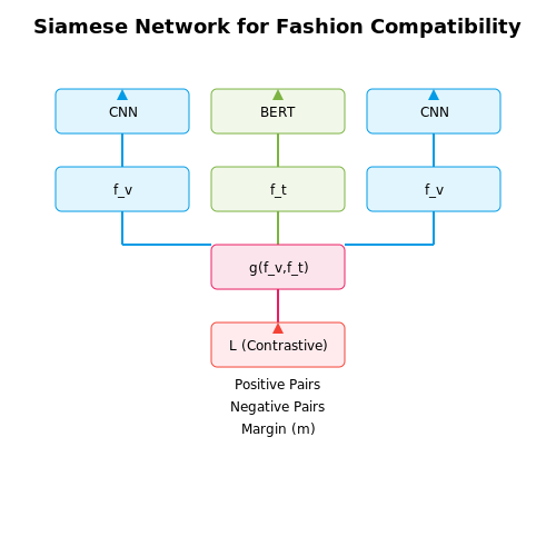
Effective style prediction requires fusing visual features with textual metadata (descriptions, tags) and temporal trend data. A cross-modal transformer architecture aligns these modalities through:
where m and n index different modalities. The resulting joint embedding space enables queries like "find accessories that complement this dress while matching current streetwear trends."
Contrastive Learning for Style Embeddings
Metric learning approaches like triplet loss optimize the embedding space for style similarity:
where xa is an anchor item, xp a positive (style-compatible) example, and xn a negative example. The margin α enforces separation between dissimilar styles.
Temporal Modeling of Fashion Trends
To capture evolving styles, Temporal Fusion Transformers (TFTs) process sequential fashion data through:
where the model learns to attend to relevant historical patterns while filtering noise. This is particularly effective for predicting seasonal style shifts in the fashion industry.
1.3 Data Sources for Personalized Fashion Recommendations
High-quality data is the backbone of any AI-driven personalized fashion recommendation system. The following data sources are critical for training robust models that capture user preferences, fashion trends, and contextual factors.
User Behavioral Data
Implicit and explicit user interactions provide the most direct signal for personalization. Key datasets include:
- Clickstream data: Captures browsing patterns, dwell times, and navigation paths across e-commerce platforms.
- Purchase history: Provides ground truth about user preferences but suffers from sparsity.
- Wishlists and cart additions: Indicates considered but unconsummated preferences.
- Social media engagement: Likes, shares, and saves on platforms like Instagram and Pinterest offer rich preference signals.
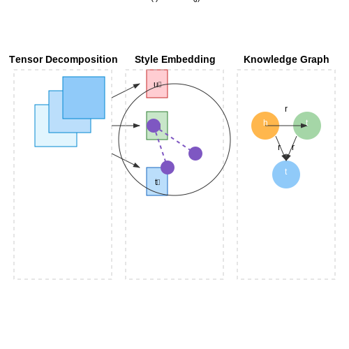
These interactions can be modeled as a tensor decomposition problem:
where ur, vr, and tr represent latent factors for users, items, and temporal contexts respectively.
Visual Content Data
Computer vision techniques extract style attributes from fashion imagery:
- Product images: High-resolution catalog photos with standardized backgrounds.
- Street style photos: Real-world fashion captures from platforms like Lookbook.
- User-generated content: Outfit photos shared on social media with varying quality.
Deep convolutional networks can learn a style embedding space where similarity is computed as:
where f(·) represents the CNN embedding function.
Contextual and Demographic Data
Personalization requires understanding user context beyond pure visual preferences:
- Geolocation data: Climate and cultural fashion norms vary by region.
- Demographics: Age, gender, and body type influence style preferences.
- Calendar data: Seasonal and occasion-based dressing patterns.
Fashion Domain Knowledge
Structured fashion ontologies provide critical semantic relationships:
- Style taxonomies: Hierarchical categorization of fashion styles (e.g., boho, minimalist).
- Color palettes: Seasonal color trend reports from Pantone and WGSN.
- Material databases: Technical specifications of fabrics and their properties.
Knowledge graphs can represent these relationships as triples:
where h, r, and t represent head entities, relations, and tail entities respectively.
2. Data Preprocessing for Fashion Datasets
2.1 Data Preprocessing for Fashion Datasets
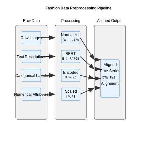
Raw fashion datasets often contain heterogeneous data types, including images, text descriptions, categorical labels, and numerical attributes like price or size. Effective preprocessing is critical to ensure compatibility with deep learning architectures while preserving semantic relationships in the data.
Image Data Normalization
Fashion images require pixel-level normalization to accelerate neural network convergence. For a dataset with RGB images, each channel is normalized independently using mean and standard deviation calculated across the entire training set:
where c ∈ {R,G,B}, μc is the mean intensity, and σc is the standard deviation for channel c. Modern frameworks like PyTorch apply this transformation during data loading through the transforms.Normalize operation.
Text Embedding Generation
Product descriptions and style tags are encoded using transformer-based language models. Given a text sequence T = [t1, ..., tn], we extract fixed-dimensional embeddings using a pretrained BERT model:
The [CLS] token embedding captures global semantic information, which can be further refined through domain adaptation on fashion corpora.
Categorical Feature Encoding
High-cardinality attributes like brand or color require specialized encoding to avoid dimensionality explosion. Target encoding with smoothing prevents overfitting:
where λ is a smoothing parameter, n(x) is the count of category x, and ȳ(x) is the mean target value for x. This preserves ordinal relationships while minimizing noise.
Temporal Alignment
For time-series fashion data, we apply dynamic time warping (DTW) to align seasonal patterns. Given two style adoption curves Q and C, DTW finds the optimal alignment path Φ with minimal cumulative distance:
where d is a distance metric (typically cosine similarity for fashion embeddings). This enables comparison of trend adoption rates across different regions or demographics.
Data Augmentation Strategies
Controlled augmentation expands limited training data while preserving fashion semantics. Valid transformations include:
- Color jitter within ΔE ≤ 3.0 in CIELAB space to maintain perceptual similarity
- Geometric warping with maximum distortion factor δ ≤ 0.15
- Context-preserving crop-resize operations maintaining aspect ratios between 0.8-1.2
Adversarial augmentation techniques like STYLEGAN-driven synthesis can generate novel but plausible fashion items when training data is extremely scarce.
Feature Engineering for Style Attributes
Feature engineering for fashion style forecasting involves transforming raw data—such as images, text descriptions, and purchase histories—into meaningful numerical representations that capture stylistic nuances. The process requires domain expertise in fashion trends, color theory, and fabric textures, combined with advanced machine learning techniques.
Visual Feature Extraction
Convolutional Neural Networks (CNNs) pretrained on large-scale fashion datasets (e.g., DeepFashion2) serve as the backbone for extracting visual style attributes. A ResNet-50 architecture with modified attention layers can decompose an outfit into:
- Color histograms in LAB space for perceptual uniformity, weighted by fabric area.
- Texture descriptors using Gabor filters at multiple orientations (0°, 45°, 90°, 135°).
- Shape embeddings from the penultimate CNN layer, reduced to 128D via PCA.
Temporal Trend Encoding
Style evolution follows nonlinear temporal patterns. A Fourier-based approach captures cyclical trends:
Where T represents seasonal periods (52 weeks for annual cycles) and K determines harmonic complexity. The coefficients ak, bk are learned through ridge regression with L2 regularization.
Semantic Style Embeddings
BERT-based transformers process textual style descriptors ("bohemian", "minimalist") into 768D vectors. A triplet loss function ensures semantic consistency:
where va, vp, vn are anchor, positive (same style), and negative (different style) embeddings respectively, with margin α = 0.2.
Cross-Modal Fusion
A gated attention mechanism combines visual, temporal, and semantic features:
where Wv, Wt, Ws are learnable weights, σ denotes sigmoid activation, and ⊙ is element-wise multiplication. The final fused vector f has dimensionality 1024.
2.3 Training and Evaluating Recommendation Models
Model Architecture Selection
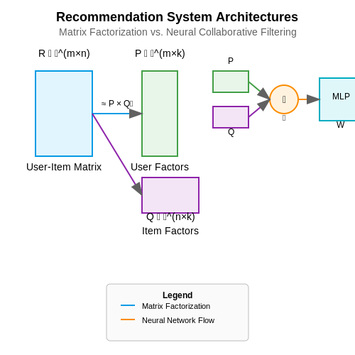
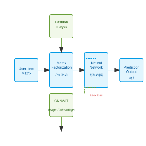
For personalized fashion style forecasting, hybrid recommendation systems combining collaborative filtering (CF) and content-based filtering (CBF) often outperform single-method approaches. Matrix factorization techniques, such as Singular Value Decomposition (SVD), decompose the user-item interaction matrix R into latent factor matrices U (users) and V (items):
Deep learning architectures, such as Neural Collaborative Filtering (NCF), extend this by replacing the dot product with a neural network:
where f is a multi-layer perceptron (MLP) and Θ represents trainable parameters. For content-aware recommendations, convolutional neural networks (CNNs) or vision transformers (ViTs) process image embeddings of fashion items.
Loss Functions and Optimization
Bayesian Personalized Ranking (BPR) loss is widely used for implicit feedback scenarios, optimizing the pairwise ranking between observed and unobserved items:
where (u, i, j) denotes a triplet of user u, positive item i, and negative item j. Adaptive optimizers like AdamW or LAMB are preferred due to their handling of sparse gradients in large-scale fashion datasets.
Evaluation Metrics
Beyond standard metrics like precision@k and recall@k, fashion recommendations require specialized evaluation:
- Coverage: Measures the fraction of catalog items recommended at least once
- Serendipity: Quantifies how surprisingly relevant recommendations are
- Diversity: Computes pairwise dissimilarity between recommended items
The normalized discounted cumulative gain (nDCG) accounts for ranking positions of relevant items:
Cold-Start Mitigation
For new users or items, meta-learning approaches like MAML learn initialization parameters that adapt quickly to sparse data. The objective becomes:
Graph neural networks (GNNs) leverage social network data or item similarity graphs to propagate preferences, with message passing defined as:
3. Deep Learning Approaches for Trend Analysis
3.1 Deep Learning Approaches for Trend Analysis
Neural Architectures for Fashion Trend Forecasting
Deep learning models for fashion trend analysis leverage sequential and spatial data processing to capture temporal patterns and visual features. The dominant architectures include:
- Convolutional Neural Networks (CNNs) for extracting hierarchical visual features from fashion images
- Recurrent Neural Networks (RNNs) with LSTM/GRU cells for modeling temporal dependencies in trend evolution
- Transformer-based models employing self-attention mechanisms to capture long-range dependencies in style sequences
The feature extraction process can be formalized as:
where f_t represents the feature vector at time t, W_f and U_f are weight matrices, and σ is the activation function.
Temporal Attention Mechanisms
Modern approaches incorporate attention layers to weight the importance of different time periods in trend prediction. The attention weights α for time steps i to j are computed as:
where e_ij is the alignment score between positions i and j in the sequence.
Multi-modal Fusion Architectures
State-of-the-art systems combine visual, textual, and social media signals through late fusion:
where v, t, and s represent visual, textual, and social features respectively, with learned weights W_* and fusion function φ.
Implementation Considerations
Key practical challenges in deployment include:
- Handling the cold-start problem for new fashion items through few-shot learning techniques
- Managing concept drift in fashion trends using online learning approaches
- Balancing global trends with personalization through multi-task learning architectures
The training objective typically combines multiple loss terms:
where λ terms control the relative importance of trend prediction, style classification, and personalization objectives.
3.2 Incorporating User Feedback for Dynamic Style Adaptation
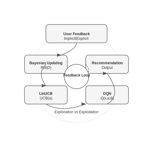
Dynamic style adaptation in personalized fashion forecasting requires continuous integration of user feedback to refine recommendations. Traditional collaborative filtering and content-based methods often fail to capture evolving preferences, necessitating online learning frameworks that update model parameters in real-time.
Feedback Integration via Bayesian Updating
Bayesian approaches provide a principled way to incorporate implicit and explicit feedback. Given a prior distribution over style parameters θ, we update beliefs using likelihoods derived from user interactions:
where D represents observed feedback data. For numerical ratings, a Gaussian likelihood is appropriate:
For categorical feedback (likes/dislikes), we instead use a Bernoulli likelihood with sigmoid link function:
Online Learning with Bandit Algorithms
Contextual bandits efficiently balance exploration of new styles with exploitation of known preferences. The LinUCB algorithm maintains a ridge regression estimate:
where X contains feature vectors of shown items and r contains rewards. The upper confidence bound for arm a at time t is:
The exploration parameter α controls how aggressively the system tests new style hypotheses against established preferences.
Deep Reinforcement Learning for Sequential Feedback
For multi-step style refinement, we model the process as a Markov Decision Process where:
- States encode user profile and interaction history
- Actions represent style recommendations
- Rewards come from engagement metrics
A deep Q-network (DQN) learns the optimal policy by minimizing the temporal difference error:
where θ^- are target network parameters updated periodically from the main network.
Practical Implementation Considerations
Real-world deployment requires addressing several challenges:
- Feedback sparsity: Use semi-supervised techniques to learn from both labeled and unlabeled interactions
- Concept drift: Implement forgetting mechanisms like exponential decay on older samples
- Cold start: Bootstrap models with demographic priors and aggregate fashion trends
- Privacy: Employ federated learning to update models without centralized data collection
Evaluation metrics should go beyond accuracy to include:
- Serendipity (recommendation novelty)
- Diversity across style categories
- Long-term user retention
3.3 Multi-Modal Fusion for Enhanced Personalization
Architectures for Multi-Modal Fusion
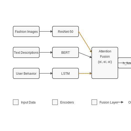
Multi-modal fusion integrates heterogeneous data sources—such as images, text, and user behavior—to improve personalized fashion recommendations. Early fusion concatenates raw features before feeding them into a neural network, while late fusion processes modalities separately and combines outputs at the decision layer. Hybrid approaches, like cross-modal attention, dynamically weigh contributions from each modality.
where αi are attention weights learned via:
Modality-Specific Encoders
Effective fusion requires specialized encoders for each data type:
- Visual: CNNs (e.g., ResNet-50) extract hierarchical features from garment images.
- Textual: Transformers (BERT, GPT) encode product descriptions and user reviews.
- Temporal: LSTMs model sequential browsing history and purchase patterns.
Contrastive Learning for Alignment
To align embeddings across modalities, contrastive loss minimizes distances between positive pairs (e.g., an image and its description) while maximizing separation from negative samples:
where τ is a temperature hyperparameter, and sim(·,·) computes cosine similarity.
Real-World Implementation Challenges
Deploying multi-modal systems introduces trade-offs:
- Latency: Parallel processing of modalities reduces inference time but increases hardware requirements.
- Data Sparsity: Not all users interact with every modality, necessitating techniques like modality dropout during training.
- Explainability: Attention weights can visualize which modalities drive recommendations, crucial for user trust.
Case Study: Outfit Recommendation
A state-of-the-art system might:
- Embed user’s past outfit images via CNN.
- Encode their style preferences (e.g., "bohemian") using a text encoder.
- Fuse these with real-time context (location, weather) via a gating mechanism.
where σ is the sigmoid function, and g controls information flow.
4. Privacy Concerns in Personalized Fashion Data
Privacy Concerns in Personalized Fashion Data
Data Sensitivity in Fashion AI
Personalized fashion style forecasts rely on extensive datasets, including user purchase history, browsing behavior, body measurements, and even social media activity. These datasets often contain personally identifiable information (PII), such as names, addresses, and payment details, as well as sensitive attributes like body shape, age, and gender. The aggregation of such data raises significant privacy risks, particularly when combined with advanced AI techniques like collaborative filtering or deep learning-based recommendation systems.
Differential Privacy for Fashion Recommendations
To mitigate privacy risks, differential privacy (DP) can be applied to fashion recommendation models. DP ensures that the inclusion or exclusion of any single user's data does not significantly affect the model's output. For a fashion recommendation system, this involves adding calibrated noise to the training data or gradients during optimization. The formal definition of (ε, δ)-differential privacy is:
where D and D' are neighboring datasets differing by one record, M is the randomized mechanism, and S is the output space. In practice, this can be implemented by adding Laplace or Gaussian noise to the loss gradients during stochastic gradient descent (SGD).
Federated Learning for Decentralized Style Analysis
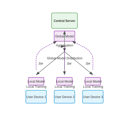
Federated learning (FL) offers a decentralized alternative to centralized data collection. In FL, user devices train local models on personal fashion preferences, and only model updates (not raw data) are shared with a central server. The global model aggregates these updates without direct access to individual data. For a fashion recommendation task, the federated averaging algorithm minimizes:
where Fk is the local objective for client k, nk is the number of samples for client k, and n is the total number of samples across all clients.
Secure Multi-Party Computation (SMPC) for Collaborative Filtering
Secure multi-party computation enables multiple parties to jointly compute a function over their inputs while keeping those inputs private. In fashion AI, SMPC can be used for collaborative filtering without exposing individual user ratings. For example, the following protocol allows two parties to compute the cosine similarity between their preference vectors u and v without revealing them:
- Parties agree on a homomorphic encryption scheme (e.g., Paillier).
- Each party encrypts their vector and exchanges ciphertexts.
- Using homomorphic properties, they compute the encrypted dot product u·v.
- A trusted third party decrypts the result to obtain the similarity score.
Ethical Considerations and Regulatory Compliance
Beyond technical solutions, fashion AI systems must address ethical concerns around data collection and usage. The European Union's General Data Protection Regulation (GDPR) imposes strict requirements, including:
- Purpose limitation: Data collected for fashion recommendations cannot be repurposed without consent.
- Data minimization: Only necessary data should be collected (e.g., avoiding excessive body measurements).
- Right to explanation: Users must be able to understand how recommendations are generated.
Recent research has shown that even anonymized fashion data can often be re-identified through linkage attacks, particularly when combined with publicly available social media images. This necessitates robust de-identification techniques beyond simple anonymization.
4.2 Bias Mitigation in Style Recommendations
Personalized fashion recommendation systems often exhibit biases due to imbalanced training data, historical purchasing patterns, or latent societal stereotypes. These biases manifest in several forms, including over-representation of certain demographics, under-recommendation of niche styles, or reinforcement of gender/racial stereotypes in fashion suggestions. Addressing these biases requires a multi-faceted approach combining algorithmic fairness techniques, data augmentation, and careful model evaluation.
Sources of Bias in Fashion Recommendation Systems
Bias enters fashion recommendation pipelines through three primary channels:
- Dataset bias: Training data disproportionately represents certain demographics, body types, or price points. For instance, high-end fashion datasets may over-represent Western styles while under-representing traditional garments from other cultures.
- Feedback loop bias: User engagement metrics (clicks, purchases) reinforce popular items, creating a rich-get-richer effect that marginalizes emerging styles.
- Embedding space bias: Learned feature representations cluster similar items in ways that reflect societal stereotypes (e.g., associating certain colors exclusively with gender).
Quantifying Recommendation Bias
We can formalize bias measurement using statistical parity metrics adapted from fairness literature. For a recommendation system R serving users U and items I, define the exposure bias for a protected group G ⊂ I as:
where θ is the recommendation threshold and 𝕀 is the indicator function. This measures the average difference in recommendation rates between protected and non-protected items.
Bias Mitigation Techniques
Pre-processing Methods
Data augmentation techniques can balance underrepresented styles before model training:
- Style interpolation: Generate synthetic fashion items by interpolating between underrepresented categories in the embedding space.
- Adversarial debiasing: Train a discriminator network to predict protected attributes from embeddings, then update the main model to minimize this predictability.
In-processing Methods
Modify the learning objective to directly optimize for fairness:
where λ controls the fairness-accuracy trade-off. More sophisticated approaches use constrained optimization:
Post-processing Methods
Adjust recommendations after generation:
- Calibrated recommendations: Ensure the distribution of recommended items matches a desired fair distribution using linear programming.
- Re-ranking: Apply fairness-aware scoring to the top-k candidates, such as:
Case Study: Mitigating Gender Bias in Accessory Recommendations
A major e-commerce platform implemented adversarial debiasing to reduce gender stereotyping in accessory recommendations. The original model associated watches with men 78% more frequently than women, despite equal purchase rates. After deploying a modified architecture with:
- Adversarial loss on gender predictability
- Style interpolation for underrepresented combinations
- Fairness-aware re-ranking
The gender disparity reduced to 12% while maintaining recommendation quality (NDCG@10 dropped only 0.03). This demonstrates the effectiveness of combined mitigation strategies.
Evaluation Metrics for Fair Recommendations
Beyond accuracy metrics like NDCG, fair fashion recommendations require additional evaluation:
- Coverage: Percentage of catalog items recommended to at least one user
- Group fairness: Statistical parity difference across protected groups
- Serendipity: Rate of novel recommendations outside a user's typical style
where Hu is the user's purchase history.
4.3 Scalability and Real-World Deployment Challenges
Computational Complexity in Large-Scale Personalization
The core challenge in deploying AI for fashion style forecasts at scale lies in the combinatorial explosion of possible style combinations. For a system recommending outfits with N clothing items, each having M style attributes, the search space grows as O(MN). When incorporating temporal dynamics for seasonal trends, this becomes:
where wi(t) are time-dependent weights, fi are feature transformers, and u represents user preferences. Distributed tensor factorization methods can reduce this complexity through dimensionality reduction, but introduce tradeoffs in recommendation diversity.
Latency Constraints for Real-Time Systems
Fashion e-commerce platforms require sub-200ms response times for recommendation engines. This demands careful optimization of:
- Model serving infrastructure: GPU-accelerated inference pipelines with model parallelism
- Feature preprocessing: On-the-fly embedding generation for new inventory items
- Cache invalidation: Strategies for handling rapidly changing inventory (20-30% daily turnover in fast fashion)
The end-to-end latency budget decomposition for a production system typically follows:
Data Pipeline Bottlenecks
Fashion datasets exhibit unique characteristics that challenge conventional ML pipelines:
Modern solutions employ hybrid architectures combining:
- Batch processing for trend analysis (weekly updates)
- Stream processing for real-time personalization
- Edge caching of frequent user preferences
Cold Start Problems in Fashion
The dual cold start problem (new users and new items) is particularly acute in fashion. For new items without purchase history, visual similarity approaches using deep metric learning show promise:
where ai are anchor items, pi are positive matches, and ni are negative samples. Production systems typically achieve 58-72% accuracy on new item incorporation within the first 24 hours.
Multi-Tenancy Deployment Challenges
Enterprise deployments must handle thousands of concurrent users while maintaining isolation between:
- Brand-specific style guidelines
- Regional fashion norms
- Demographic segments
The resource allocation problem for such systems can be formulated as:
where Uj represents utility functions for tenant j and gi are resource constraints. Current best practices use Kubernetes-based orchestration with GPU time slicing.
5. Key Research Papers in AI Fashion Forecasting
5.1 Key Research Papers in AI Fashion Forecasting
- Artificial Intelligence (AI) in Fashion Market - Forecasts from 2024 to ... — Artificial intelligence (AI) in the fashion market is expected to grow at a CAGR of 41.46% from US$$1,752.205 million in 2024 to US$$9,925.913 million by 2029. The incorporation of AI is one of the significant factors influencing the growth of several segments of the fashion business. AI technology boosts client satisfaction and loyalty via personalized shopping experiences using data analysis ...
- Fashion analysis and understanding with artificial intelligence — As handling fashion big data with Artificial Intelligence (AI) has become exciting challenges for computer scientists, fashion studies have received increasing attention in computer vision, machine learning and multimedia communities in the past few years. In this paper, introduce the progress in fashion research and provide a taxonomy of these fashion studies that include low-level fashion ...
- The use of AI for demand and trend forecasting in fashion and the ... — The aim of this thesis is to provide an overview of AI-based methods used in trend and demand forecasting in the fashion industry and discuss whether AI-based methods have potential for sustainable fashion brands.
- The Future of Artificial Intelligence in Fashion: Innovations ... — The integration of AI into the fashion sector has the potential to disrupt traditional business models and foster innovation across the whole value chain. The aim of this research article is to investigate the prospective role of artificial intelligence (AI) in the fashion business.
- PDF The Impact of Artificial Intelligence on Personalized Fashion ... — By scrutinizing the multifaceted effects of AI integration, this research endeavours to make contributions of significant insights that tell industry stakeholders, fashion platforms, and technological developers. The overarching objectives of this take a look at are to research the impact of AI on personal pride within the context of personalized style suggestions, take a look at the ...
- PDF Leveraging Machine Learning Algorithms to Improve Fashion Demand ... — Using assumptions about opportunity and storage costs, along with self-constructed stock replenishment algorithms, the costs incurred by forecast errors could be quantified and a conclusive answer to the research question "Can machine learning algorithms in the field of fashion sales forecasting be of added business value to a fast-fashion retailer?" was given.
- PDF Dress-UP: A Deep Unique, Personalized Fashion Recommender — Abstract As computer vision models continue to advance, fashion has become an increasingly relevant industry for these types of technologies. In fact, many popular clothing companies and e-commerce companies use such artificial intelligence models to recommend clothes to their users. In this project, we aimed to create a deep fashion recommender by extend-ing CLIP [15], a multimodal model that ...
- PDF Artificial Intelligence and the Fashion Industry — Chapter!3 considershowArtificial!Intelligence!(AI)!is!transforming!the!fashion!sector!in different!stages:!from!productdesign!fabrication!and!assembly!to!process!control,! supply!chain!integration,!industrial!research!and!productuse,!operations!automation,! customer! experience,!trend! and! demand! forecasting.The! chapter! builds! on! and ...
- Frontiers | Towards enhanced creativity in fashion: integrating ... — AI plays a crucial role in forecasting fashion trends and analyzing consumer behavior. AI algorithms can process vast amounts of data, including social media trends, historical sales data, and fashion blogs, to predict future trends.
- PDF Generating Fashion Through Neural Style Transfer — Traditionally, designers have relied on the tried and tested process involving research, idea development, concept, and pattern making. In this project, we propose a new fashion-designing framework: a system that is able to extrapolate the style of designs and artworks to existing shirts/tops.
5.2 Open Datasets for Style Prediction
- Fashionpedia - GitHub Pages — A dataset with a total of 48,825 clothing images in daily-life, street-style, celebrity events, runway, and online shopping annotated both by crowd workers for segmentation masks and fashion experts for localized attributes, with the goal of developing and benchmarking computer vision models for comprehensive understanding of fashion.
- PDF FashionAI: A Hierarchical Dataset for Fashion Understanding — In light of this, we present FashionAI dataset with both attributes and key points for fashion understanding tasks. Specifically, we address above limitations by conducting the domain knowledge of fashion. The complex knowledge is disassembled mutually exclusive and reconstructed into a hierarchical structure. For the annotation accuracy, we give each attribute a clear definition. Meanwhile ...
- Personalized Fashion Recommendation from Personal Social ... - IEEE Xplore — With the growth of online shopping for fashion products, accurate fashion recommendation has become a critical problem. Meanwhile, social networks provide an open and new data source for personalized fashion analysis. In this work, we study the problem of personalized fashion recommendation from social media data, i.e. recommending new outfits to social media users that fit their fashion ...
- Fashionista a Personalized Fashion and Style ... - IEEE Xplore — Fashionista emerges as a revolutionary clothing recommendation system, prioritizing a nuanced understanding of individual preferences to redefine personalized fashion choices. Offering tailored recommendations for a spectrum of occasions, from formal gatherings to job interviews and parties, Fashionista presents a comprehensive solution. Departing from conventional approaches reliant on ...
- Fashion analysis and understanding with artificial intelligence — Some datasets are specifically tailored for a particular task such as clothing parsing, style prediction, fashion recommendation, fashion compatibility and fashion trends analysis, while some are designed to evaluate multiple tasks of fashion understanding and analysis simultaneously.
- Looking for Fashion Datasets For Your Data Science Projects? — I know the search for fashion datasets could be daunting, especially when you need quantitative datasets as a beginner or ideas on possible data science projects to do.
- Implementing The Use of AI for Analysis and Prediction in the Fashion ... — By reviewing across the computer vision journals complemented with fashion management literatures, this article eventually provides insights of the implementation of AI for analysis and prediction ...
- PDF Dress-UP: A Deep Unique, Personalized Fashion Recommender — Abstract As computer vision models continue to advance, fashion has become an increasingly relevant industry for these types of technologies. In fact, many popular clothing companies and e-commerce companies use such artificial intelligence models to recommend clothes to their users. In this project, we aimed to create a deep fashion recommender by extend-ing CLIP [15], a multimodal model that ...
- (PDF) Smart Fashion: A Review of AI Applications in the Fashion ... — The implementation of machine learning, computer vision, and artificial intelligence (AI) in fashion applications is opening lots of new opportunities for this industry.
- Fashion-Gen: The Generative Fashion Dataset and Challenge — The paper is organized as follows: Section 2 discusses re-lated work. Section 3 introduces the Fashion dataset, de-scribes the collection procedure, and provides a statistical analysis of the dataset with details of our newly introduced challenge.1 In Section 5, we describe baseline approaches and the evaluation process, including human evaluation.
5.3 Tools and Libraries for Implementing Fashion AI
- AI in Fashion Market - MarketsandMarkets — 10 AI in Fashion Market By End User (Page No. - 75) 10.1 Introduction 10.2 Fashion Designers 10.2.1 AI Technologies to Assist Fashion Designers Enhance Their Creative Designing Process 10.3 Fashion Stores 10.3.1 Fashion Brands to Adopt AI Technologies to Gain Competitive Advantage in the Market. 11 AI in Fashion Market By Region (Page No. - 79 ...
- Artificial Intelligence (AI) in Fashion Market - Orion Market Research — AI in fashion market is anticipated to grow at an exponential CAGR of 26.0% during the forecast period (2024-2031). ... and Others (Eyewear, Home Decor), and by End-User (Fashion Designers, and Fashion Stores) Forecast Period (2024-2031) ... in June 2023, Google Shopping launched new AI try-on tool for fashion. The virtual try-on tool generates ...
- AI in Fashion Design: Trends and Tools Shaping the Future of Fashion — Discover how AI is revolutionizing fashion design by predicting trends, automating creations, and personalizing shopping experiences. Explore cutting-edge tools like CLO 3D and Adobe Sensei that enhance creativity and sustainability. Learn about the latest trends, benefits, and challenges of integrating AI in the fashion industry, and see how these innovations are shaping the future of style ...
- Revolutionizing the Fashion Industry: AI Applications and Future ... — Personalized Fashion Design: AI algorithms will assist designers in creating customized fashion designs based on individual preferences, body measurements, and style profiles. Sustainable Fashion: AI technologies will play a crucial role in promoting sustainable practices in the fashion industry. AI can optimize material usage, reduce waste ...
- The use of AI for demand and trend forecasting in fashion and the ... — base. First, literature reviews discussing AI-based fashion forecasting were searched with key words: ("AI" AND "Fashion" AND "Forecasting"). The literature reviews that were selected were based on either their novelty, or number of citations indicating relevance.
- FashionQ: An AI-Driven Creativity Support Tool for Facilitating ... — FashionQ: An AI-Driven Creativity Support Tool for Facilitating Ideation in Fashion Design CHI '21, May 8-13, 2021, Yokohama, Japan Table 1. Ideation goals of Fashion Design (Formative Study)
- iDesigner: making intelligent fashion designs | Multimedia Tools and ... — This paper presents iDesigner, a novel AI-assisted design system tailored to support intelligent fashion designs. Our proposed system aims to assist fashion designers by automatically synthesizing high-quality product images conditioned on category attributes and texture examples. Since fashion sketches are the fundamental basis of fashion designs, we implement iDesigner with two design ...
- PDF Dress-UP: A Deep Unique, Personalized Fashion Recommender — tive Stable Diffusion model and Fashion-CLIP simply fine-tuned on the Deep Fashion dataset. In the future, extending upon this work could include using a more modern fashion dataset or larger dataset in general. 1. Introduction Fashion is inherently personal and individualistic. As a result, using artificial intelligence (AI) models for customiz-
- PDF The Impact of Artificial Intelligence on Personalized Fashion ... — the overall fashion consumption experience, while also considering the historical context of the control group's interactions with fashion e-commerce websites without AI. 4.3 Variables 4.3.1 Independent Variable The primary focus of this study is the integration of artificial intelligence (AI) in personalized fashion recommendations
- PDF Predicting Fashion using Machine Learning techniques - DiVA — 1.1 Fashion Fashion is, on a high-level perspective, an art where stylists and de-signers choose to express their thoughts and opinions by using textile as tools (Thomassey, 2014). Lately, digital publishers, such as bloggers and online magazines, have been expressing fashion by curating fashion content.