Manipulation Planning for Robotic Arms
1. Kinematics and Dynamics of Robotic Arms
Kinematics and Dynamics of Robotic Arms
Forward and Inverse Kinematics
The kinematic analysis of robotic arms involves two fundamental problems: forward kinematics (FK) and inverse kinematics (IK). FK computes the end-effector position and orientation given joint angles, while IK solves for joint angles that achieve a desired end-effector pose. For an n-degree-of-freedom (DOF) serial manipulator, the FK problem is straightforward through homogeneous transformation matrices:Velocity Kinematics and Jacobian
The relationship between joint velocities q̇ and end-effector twist v is given by the manipulator Jacobian J(q):Dynamics Formulation
The equations of motion for a robotic arm can be derived using Lagrangian mechanics or the Newton-Euler recursive formulation. The standard form is:Practical Considerations
- Payload variations require adaptive inertia matrix estimation
- Joint flexibility introduces additional dynamics that may necessitate state augmentation
- Friction effects (Coulomb, viscous) often dominate at low velocities
Trajectory Generation
Smooth motion planning requires time-parameterized trajectories satisfying boundary conditions on position, velocity, and acceleration. Quintic polynomials are commonly used for joint-space trajectories:Dynamic Simulation
The Featherstone algorithm provides an efficient O(n) method for forward dynamics simulation by propagating articulated-body inertias through the kinematic tree. This is implemented in physics engines like Bullet and MuJoCo for contact-rich manipulation scenarios. The articulated-body algorithm computes accelerations from applied torques without explicitly forming the system mass matrix.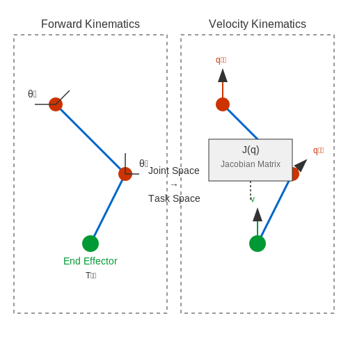
Workspace and Configuration Space Analysis
Fundamental Definitions
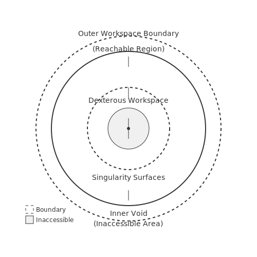
The workspace of a robotic arm refers to the set of all positions and orientations that the end-effector can reach in the physical environment. For an n-degree-of-freedom (DOF) manipulator, this is typically a subset of SE(3) (Special Euclidean Group in 3D space). The workspace can be decomposed into:
- Reachable workspace: All points the end-effector can reach with at least one orientation
- Dexterous workspace: Points reachable with all possible orientations
The configuration space (C-space) is the set of all possible joint configurations, represented as a manifold where each point corresponds to a unique joint state. For a revolute joint, this is typically S1 (a circle), while prismatic joints contribute ℝ dimensions.
Topological Properties
The C-space topology determines motion planning complexity. Key properties include:
- Connectivity: Whether the space is path-connected (any two configurations can be connected)
- Compactness: Whether the space is bounded (critical for optimization)
- Obstacle representation: Obstacles in workspace map to C-obstacles in C-space
The C-obstacle region 𝒞obs is defined as:
where 𝒜(q) is the robot geometry at configuration q and 𝒪 represents workspace obstacles.
Dimensionality and Representation
For an n-DOF manipulator, C-space is n-dimensional. Common representations include:
- Explicit parameterization: Direct joint angle/position coordinates
- Implicit representation: Using constraint equations
- Quaternion space: For orientation components (avoiding gimbal lock)
The workspace-to-configuration mapping is given by the forward kinematics function:
Practical Computation Methods
For real-world applications, several computational approaches are employed:
Sampling-Based Analysis
Monte Carlo methods generate workspace points by sampling random configurations:
where U(𝒞) is uniform sampling over C-space.
Algebraic Decomposition
For simple manipulators, workspace boundaries can be derived analytically. For example, a 2R planar arm has workspace boundaries at:
Case Study: 6-DOF Industrial Arm
Consider a typical 6R manipulator (e.g., UR5, KUKA KR6). Its C-space is:
The workspace forms a complex 3D volume with:
- Inner void where end-effector cannot reach
- Singularity surfaces where mobility is reduced
- Multiple inverse kinematic solutions per workspace point
Degrees of Freedom and Redundancy
Kinematic Degrees of Freedom
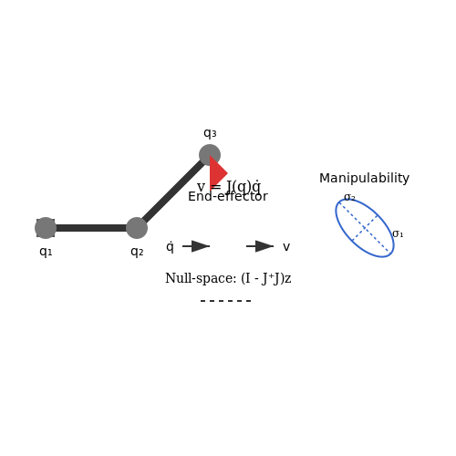
The degrees of freedom (DoF) of a robotic arm represent the number of independent parameters required to fully specify its configuration in space. For a serial-chain manipulator, this equals the number of actuated joints. A rigid body in 3D space has 6 DoF (3 positional, 3 rotational), so a manipulator requires at least 6 joints to achieve arbitrary end-effector poses. The Jacobian matrix J(q) relates joint velocities q̇ to end-effector twist v:
When J(q) is square (non-redundant case), instantaneous motion planning reduces to solving this linear system. However, when the Jacobian becomes rank-deficient (at singular configurations), certain end-effector motions become impossible.
Redundancy Resolution
A manipulator is kinematically redundant when it possesses more DoF than required for a task. For spatial positioning (3D), any arm with >3 joints is redundant; for full pose control (6D), >6 joints create redundancy. This excess enables:
- Obstacle avoidance through null-space motions
- Optimization of secondary criteria (joint limits, energy, manipulability)
- Singularity avoidance via configuration control
The general solution for redundant systems decomposes joint velocities into:
where J+ is the Moore-Penrose pseudoinverse and z is an arbitrary vector projected into the null space of J. The term (I - J+J)z generates self-motions that change the arm's configuration without affecting end-effector pose.
Manipulability Analysis
The manipulability ellipsoid, derived from the singular value decomposition of J(q), visualizes directional motion capability. Its volume (given by √det(JJT)) quantifies dexterity. Redundant manipulators can maximize this measure through null-space optimization:
where w(q) is a manipulability metric and k0 a gain constant. This approach maintains high dexterity while executing primary tasks.
Practical Implementation Challenges
Real-world redundancy resolution must account for:
- Joint torque limits through weighted pseudoinverses
- Algorithmic singularities in extended Jacobian methods
- Task prioritization in hierarchical control schemes
The dynamically consistent pseudoinverse J# = M-1JT(JM-1JT)-1, where M is the mass matrix, ensures optimal force distribution while preserving kinetic energy properties.
2. Sampling-Based Planners (RRT, PRM)
Sampling-Based Planners (RRT, PRM)
Probabilistic Roadmaps (PRM)
Probabilistic Roadmaps (PRM) construct a graph representation of the configuration space by randomly sampling collision-free configurations and connecting them via local paths. The algorithm operates in two phases: learning and query. During the learning phase, nodes are sampled uniformly at random from the free configuration space Cfree, and edges are created between neighboring nodes if a collision-free path exists. The query phase uses standard graph search algorithms (e.g., A*) to find paths between start and goal configurations.
where μ(V) is the volume of the free space and N is the number of samples. PRM performs well in high-dimensional spaces but struggles with narrow passages due to uniform sampling.
Rapidly-Exploring Random Trees (RRT)
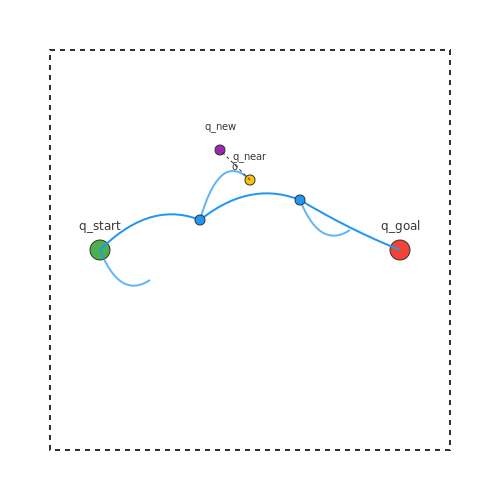
RRT grows a tree rooted at the initial configuration by iteratively expanding toward randomly sampled points. At each iteration, the algorithm:
- Samples a random configuration qrand from C.
- Finds the nearest node qnear in the tree.
- Extends from qnear toward qrand by a fixed step size δ to generate qnew.
- Adds qnew to the tree if the path between qnear and qnew is collision-free.
RRTs are probabilistically complete, meaning the probability of finding a solution approaches 1 as the number of iterations increases. Variants like RRT* asymptotically converge to optimal paths by rewiring the tree.
Practical Considerations
Key parameters influencing performance include:
- Sampling strategy: Uniform sampling may miss narrow passages; Gaussian or bridge sampling improves coverage.
- Distance metric: Euclidean distance is common, but task-specific metrics (e.g., considering robot kinematics) enhance efficiency.
- Collision checking: Optimized spatial partitioning (e.g., KD-trees) accelerates nearest-neighbor queries.
In industrial applications, PRM suits multi-query scenarios (e.g., warehouse robots), while RRT excels in single-query problems (e.g., surgical robotics). Hybrid approaches combine their strengths—PRM for global roadmaps and RRT for local refinement.
Visualization
The diagram illustrates an RRT exploring the configuration space (rectangle) from start (green) to goal (red). Blue curves represent tree branches, showing non-uniform exploration biased toward unexplored regions.
Optimization-Based Approaches
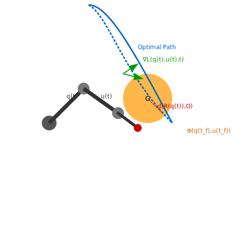
Optimization-based manipulation planning formulates the problem as a constrained numerical optimization, where the goal is to minimize an objective function while satisfying kinematic, dynamic, and task-specific constraints. These approaches leverage gradient-based or sampling-based solvers to compute trajectories that are locally or globally optimal with respect to a defined cost metric.
Mathematical Formulation
The core problem can be expressed as:
subject to:
- Kinematic constraints: \( \mathbf{q}_{\text{min}} \leq \mathbf{q}(t) \leq \mathbf{q}_{\text{max}} \)
- Dynamic constraints: \( \dot{\mathbf{q}}(t) = f(\mathbf{q}(t), \mathbf{u}(t)) \)
- Collision avoidance: \( d(\mathcal{R}(\mathbf{q}(t)), \mathcal{O}) > \epsilon \)
- Task constraints: \( g(\mathbf{q}(t), \mathbf{u}(t)) = 0 \)
where \( \mathbf{q}(t) \) is the joint configuration, \( \mathbf{u}(t) \) is the control input, \( \mathcal{L} \) is the running cost, and \( \Phi \) is the terminal cost.
Gradient-Based Optimization
Gradient-based methods, such as Sequential Quadratic Programming (SQP) or Interior-Point Optimization, iteratively refine the solution by computing the gradient of the cost function with respect to the decision variables. The update rule follows:
where \( \mathbf{x} = [\mathbf{q}, \mathbf{u}] \) is the optimization variable, \( \alpha_k \) is the step size, and \( \nabla f \) is the gradient of the cost function. These methods are efficient for high-dimensional problems but may converge to local minima.
Sampling-Based Optimization
Sampling-based approaches, such as Covariant Hamiltonian Optimization for Motion Planning (CHOMP) or Stochastic Trajectory Optimization for Motion Planning (STOMP), explore the configuration space by generating and evaluating candidate trajectories. CHOMP, for instance, minimizes the functional:
where \( \mathcal{U} \) is a smoothness prior, \( \mathcal{C} \) is the obstacle cost, and \( \xi \) is the trajectory. The update is computed using functional gradient descent:
where \( \mathbf{A} \) is a smoothing kernel matrix.
Practical Considerations
Real-world implementation requires:
- Efficient collision checking using bounding-volume hierarchies or signed distance fields.
- Warm-starting the solver with an initial feasible trajectory to improve convergence.
- Regularization to avoid singularities and numerical instabilities.
Applications include industrial assembly, where precise trajectory optimization ensures minimal cycle time while avoiding obstacles, and surgical robotics, where smooth and collision-free motion is critical.
2.3 Hybrid Planning Techniques
Hybrid planning techniques combine sampling-based and optimization-based approaches to leverage their respective strengths while mitigating weaknesses. Sampling-based methods like RRT* excel in exploring high-dimensional configuration spaces but often produce suboptimal paths, while optimization-based techniques like CHOMP generate smooth trajectories but require good initial guesses and are prone to local minima.
Mathematical Formulation of Hybrid Planning
The hybrid planning problem can be formulated as a constrained optimization where the objective is to minimize a cost function C while satisfying collision constraints Φ:
where q represents the robot's configuration. The hybrid approach typically decomposes this into two phases:
- Global exploration using sampling to find a feasible path qinit
- Local refinement through optimization to improve the path quality
STOMP-RRT Integration
A common hybrid approach combines RRT* with STOMP (Stochastic Trajectory Optimization for Motion Planning). The RRT* provides an initial collision-free path which STOMP then optimizes using stochastic sampling of control space:
where ϵ is a step size, wi are weights, and K is a kernel function that smooths the trajectory.
Constraint Handling in Hybrid Planning
Hybrid planners must handle both hard constraints (collision avoidance) and soft constraints (smoothness). The optimization phase typically uses a barrier function approach:
where λ is a weighting parameter that balances smoothness against constraint violation.
Implementation Considerations
Effective hybrid planning requires careful tuning of several parameters:
- Sampling density in the exploration phase
- Optimization step size and convergence criteria
- Constraint relaxation parameters
- Termination conditions for the refinement phase
Modern implementations often use adaptive strategies where these parameters are adjusted dynamically based on planning progress and environment complexity.
Case Study: Industrial Assembly Task
In a peg-in-hole assembly task with tight tolerances, a hybrid planner might first use RRT-Connect to quickly find an approximate path to the hole location, then switch to trajectory optimization to precisely align the peg while maintaining force constraints. This combination reduces planning time from minutes to seconds compared to pure optimization approaches while achieving higher precision than sampling alone.
The figure below illustrates this process, showing how the initial RRT path (red) is refined through optimization (blue) to produce a smooth, constraint-satisfying trajectory (green).
3. Grasp Synthesis and Stability Analysis
3.1 Grasp Synthesis and Stability Analysis
Grasp Synthesis Fundamentals
Grasp synthesis involves computing contact points and forces between a robotic hand and an object to achieve stable manipulation. The problem is formulated as finding a set of wrenches (combined force and torque vectors) that can resist external disturbances while satisfying friction constraints. For an n-finger grasp, the wrench space W is constructed as:
where Gi is the grasp matrix for contact i, and fi is the contact force vector. The grasp matrix maps local contact forces to the object's centroidal frame.
Stability Criteria
A grasp is considered stable if it satisfies two conditions:
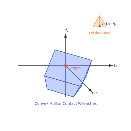
- Force closure: The convex hull of primitive contact wrenches must contain the origin of the wrench space.
- Friction constraints: Contact forces must lie within the friction cone defined by Coulomb's law: ft ≤ μfn, where μ is the friction coefficient.
The quality of a grasp can be quantified using the epsilon metric (ε), representing the radius of the largest wrench sphere centered at the origin and fully contained within the convex hull of contact wrenches:
Computational Approaches
Modern grasp synthesis algorithms typically employ one of three paradigms:
1. Analytical Methods
Solve the grasp planning problem using geometric and force-balance constraints. Common techniques include:
- Form closure tests via rank conditions on the grasp matrix
- Constructive solid geometry (CSG) for contact point generation
2. Sampling-Based Methods
Generate candidate grasps through random sampling of hand configurations, then evaluate them using stability metrics. The process involves:
- Discretization of the hand's configuration space
- Monte Carlo sampling of contact points
- Parallel evaluation of grasp quality metrics
3. Learning-Based Methods
Train neural networks to predict grasp stability from object and hand representations. State-of-the-art approaches use:
- Graph neural networks operating on point clouds
- 6D pose estimation with stability prediction heads
- Reinforcement learning for grasp refinement
Practical Implementation Considerations
Real-world grasp synthesis must account for:
- Uncertainty in object pose estimation (typically modeled as Gaussian noise in SE(3))
- Compliance in finger joints and contact surfaces
- Dynamic effects during object acquisition
The grasp stability margin S under uncertainty can be computed as:
where κ is a safety factor (typically 2-3) and σ represents the estimated uncertainty in wrench space.
3.2 Force Closure and Form Closure
Fundamental Definitions
Force closure and form closure describe two distinct mechanisms by which a robotic gripper or manipulator can constrain an object's motion. Force closure occurs when contact forces can generate any wrench (combination of forces and torques) on the object, while form closure arises when the object's motion is restricted purely by geometric constraints, even in the absence of friction.
Mathematical Characterization
For a set of n contact points, force closure is achieved if the composite wrench matrix W spans the entire wrench space. The condition is formally expressed as:
where W is constructed from the individual wrenches wi at each contact point:
For form closure, the requirement is stricter: the negative wrench space must lie strictly within the convex hull of the contact wrenches:
Practical Implications
In robotic grasping, force closure is more commonly utilized due to its reliance on friction, which allows fewer contact points (as few as two for planar cases with sufficient friction). Form closure, while more robust since it doesn't depend on friction, typically requires at least four frictionless contacts in 2D or seven in 3D, making it less practical for many applications.
Example: Two-Finger Grasp Analysis
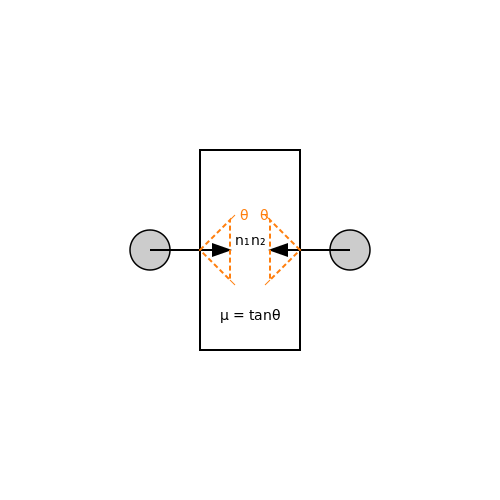
Consider a two-finger gripper with friction coefficient μ grasping a rectangular object. The force closure condition requires that the friction cones at both contacts intersect, ensuring that any external force can be counteracted by appropriate internal forces. The minimum angle θ between contact normals for force closure is given by:
This illustrates how friction enables force closure with minimal contacts, whereas form closure would require additional constraints to prevent motion without relying on friction.
Applications in Manipulation Planning
Force closure is critical in tasks requiring stable grasps under external disturbances, such as assembly or object transport. Form closure finds niche applications in fixturing and precision manipulation where friction cannot be guaranteed. Modern robotic systems often use hybrid approaches, combining geometric constraints with controlled friction to optimize grasp stability.
3.3 Task-Specific Manipulation Planning
Task-specific manipulation planning optimizes robotic arm trajectories for specialized objectives, such as assembly, grasping, or obstacle avoidance. Unlike general-purpose planners, these methods incorporate domain knowledge to improve efficiency and success rates in constrained environments.
Constraint Formulation
Task constraints are typically expressed as equality or inequality conditions on the robot's configuration space C. For a manipulator with n degrees of freedom, let q ∈ C ⊂ ℝn denote the joint angles. Common constraints include:
- End-effector pose constraints: fpose(q) = xdesired, where xdesired is the target position and orientation.
- Obstacle avoidance: d(q) > δ, with d(q) being the minimum distance to obstacles and δ a safety margin.
- Joint limits: qmin ≤ q ≤ qmax.
Task-Space Optimization
For precision tasks like peg-in-hole assembly, the operational space formulation provides better control. The task-space dynamics are derived from the joint-space dynamics using the Jacobian J(q):
where F is the operational space force and τ0 is the null-space torque. This allows decoupled control of end-effector motion and secondary objectives.
Learning-Based Approaches
Modern planners often combine optimization with machine learning. For example, a neural network can predict feasible trajectories that are then refined by a constrained optimizer:
- Train a policy πθ(qt|ot) using demonstrations or reinforcement learning.
- Use the policy outputs to warm-start a trajectory optimizer.
- Project the trajectory onto the constraint manifold using sequential quadratic programming.
Case Study: KUKA LBR iiwa Assembly
In a gear assembly task, the planner first identifies mating surfaces using a vision system, then generates a hybrid force/position trajectory. The force profile follows:
where Fcontact is adjusted based on tactile feedback to prevent jamming.
Multi-Modal Planning
Complex tasks may require switching between different manipulation modes. A screwing operation, for instance, transitions through:
- Approach: Free-space motion to pre-insertion pose.
- Search: Spiral search with force monitoring.
- Engagement: Combined axial force and rotation.
- Fastening: Constant torque control.
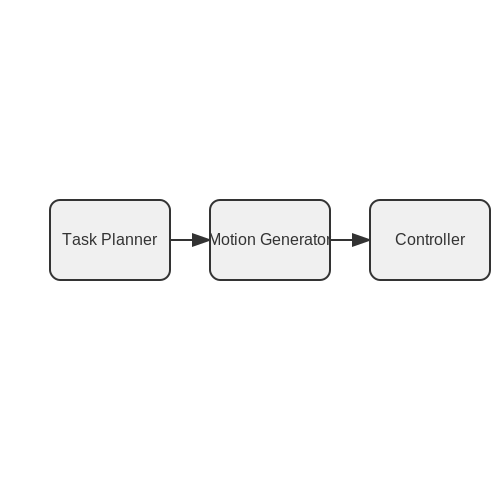
Mode transitions are triggered by sensory thresholds and governed by finite state machines. The complete planning hierarchy integrates:
Real-world implementations must account for uncertainties in perception, control, and environment dynamics. Adaptive planners use online parameter estimation to update models during execution.
4. Geometric and Sensor-Based Collision Detection
Geometric and Sensor-Based Collision Detection
Geometric Collision Detection
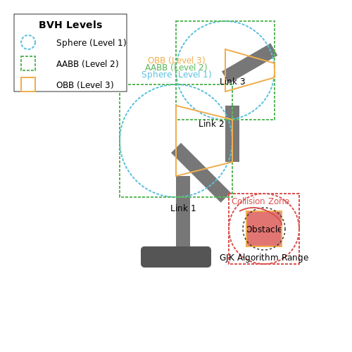
Geometric collision detection relies on mathematical representations of robotic arm links and obstacles in the workspace. The most common approach involves bounding volume hierarchies (BVH), where complex shapes are approximated using simpler geometric primitives such as spheres, axis-aligned bounding boxes (AABBs), or oriented bounding boxes (OBBs). For a robotic arm with n links, the collision check between link i and an obstacle reduces to pairwise intersection tests between their respective bounding volumes.
The Gilbert-Johnson-Keerthi (GJK) algorithm is particularly efficient for convex shapes, operating in O(n) time by iteratively reducing the problem to finding the minimum distance between two convex hulls. For non-convex objects, a decomposition into convex sub-shapes is performed prior to applying GJK.
Continuous Collision Detection
When dealing with fast-moving robotic arms, discrete collision checking at sampled time steps may miss collisions occurring between samples. Continuous collision detection (CCD) solves this by modeling the swept volume of the arm's motion. The time of impact (TOI) between two moving objects A(t) and B(t) is found by solving:
For articulated arms, this requires solving the forward kinematics for all intermediate configurations between the start and end poses. The conservative advancement technique provides an efficient solution by iteratively advancing the simulation time while ensuring no collisions are missed.
Sensor-Based Collision Detection
Geometric methods alone cannot account for unmodeled obstacles or dynamic environments. Sensor-based approaches fuse data from:
- Proximity sensors: Infrared, ultrasonic, or capacitive sensors provide distance-to-obstacle measurements
- Force-torque sensing: Detects unexpected contact forces during motion
- Vision systems: RGB-D cameras or LiDAR generate 3D point clouds of the environment
A Bayesian framework combines these sensor readings with the geometric model to estimate collision probability:
where z1:t represents the sensor measurements up to time t and η is a normalizing constant.
Implementation Considerations
Modern robotic systems often implement a hybrid approach:
- Pre-computed BVH trees for static environments
- GPU-accelerated collision checking using CUDA or OpenCL for real-time performance
- Multi-rate processing where geometric checks run at lower frequencies than sensor-based checks
The choice of collision detection method depends on the required safety level, computational constraints, and environmental dynamics. Surgical robots, for instance, require sub-millimeter accuracy and microsecond response times, while industrial arms may prioritize computational efficiency over precision.
4.2 Real-Time Collision Avoidance Techniques
Distance-Based Collision Detection
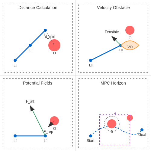
Real-time collision avoidance relies on continuous evaluation of the minimum distance between the robotic arm and obstacles. Given a robotic arm with n links and an obstacle represented as a point cloud or mesh, the minimum distance dmin is computed as:
where Li denotes the i-th link and O represents the obstacle. For polygonal meshes, the Gilbert-Johnson-Keerthi (GJK) algorithm efficiently computes the Euclidean distance between convex shapes, while expanding polytope algorithms (EPA) handle penetration depth.
Velocity Obstacles and Dynamic Constraints
Velocity obstacles extend collision avoidance to dynamic environments by predicting future collisions based on relative velocities. Given a robot configuration q and obstacle velocity vobs, the velocity obstacle cone VO is defined as:
where λ represents the robot's swept volume. The feasible velocity set FV is then FV = Vmax \ VO, where Vmax is the maximum allowable velocity.
Potential Field Methods
Artificial potential fields generate repulsive forces Frep from obstacles and attractive forces Fatt toward the goal:
where η is a scaling factor, d is the current distance, and d0 is the influence threshold. The total force Ftotal = Fatt + Frep guides the arm along collision-free paths.
Model Predictive Control (MPC) for Collision Avoidance
MPC optimizes a finite-horizon trajectory while enforcing collision constraints. The optimization problem at time step k is:
where H is the horizon length, R is a control cost matrix, and δ is a safety margin. Sequential quadratic programming (SQP) or interior-point methods solve this nonlinear program in real time.
Learning-Based Approaches
Deep reinforcement learning (DRL) trains collision-avoidance policies through reward shaping. The reward function rt often includes:
- Penalties for proximity to obstacles: robs = -exp(-α dmin)
- Goal-reaching bonuses: rgoal = β \| q - qgoal \|-1
Proximal Policy Optimization (PPO) and Soft Actor-Critic (SAC) are common DRL algorithms for this task, with point cloud or depth images as inputs.
Hardware-Accelerated Computation
GPU-accelerated libraries like CUDA and OpenCL enable real-time distance queries for complex scenes. Parallel breadth-first search (BFS) on voxel grids achieves O(1) collision checks, while k-D trees accelerate nearest-neighbor searches for point clouds.
4.3 Dynamic Environment Handling
Robotic arms operating in unstructured environments must account for dynamic obstacles, moving targets, and real-time sensor noise. Traditional motion planners assume static worlds, but dynamic scenarios require adaptive strategies that balance computational efficiency with reactivity. The core challenge lies in maintaining collision-free trajectories while responding to environmental changes within bounded latency.
Reactive Control with Velocity Obstacles
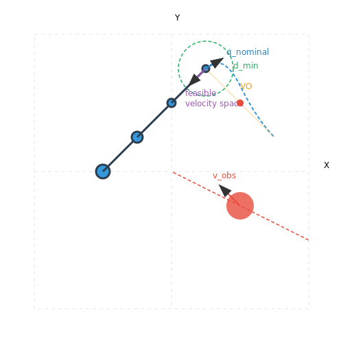
Velocity obstacles (VO) extend geometric collision checking by incorporating relative motion between the robot and dynamic objects. Given a robotic arm with joint velocities q̇ and an obstacle moving at velocity vobs, the unsafe velocity set is defined as:
where λ computes the minimum distance between the robot configuration q and obstacle O, and dmin is the safety margin. The feasible velocity space is then q̇safe = q̇nominal ∖ VO, where ∖ denotes set difference.
Temporal Planning with Spatiotemporal STL
Signal Temporal Logic (STL) enables formal specification of dynamic constraints. A trajectory ξ(t) satisfies STL formula φ = ◇[0,T] (d(ξ(t), O(t)) > r) if it maintains minimum distance r from obstacle O(t) over time horizon T. The robustness degree ρ(φ,ξ) quantifies constraint satisfaction:
STL-based optimization maximizes ρ while minimizing trajectory jerk, formulated as a nonlinear program with time-varying constraints.
Gaussian Process Motion Fields
For environments with stochastic dynamics, Gaussian processes model obstacle motion as a continuous velocity field:
where m(x) is the mean function and k(x,x') a kernel encoding spatiotemporal correlations. The probability of collision at time t becomes:
with B(q(t)) representing the robot's swept volume. Motion planners can then minimize the expected collision cost E[Pcoll] through Monte Carlo sampling of future obstacle states.
Hardware-Aware Latency Compensation
Real systems exhibit control loop delays δ between perception and actuation. The effective obstacle position becomes Ô(t) = O(t+δ), predicted via Kalman filtering or neural networks. The modified velocity obstacle formulation accounts for this prediction uncertainty:
where ⊕ is the Minkowski sum and 𝒰δ represents the prediction error ellipsoid. This ensures safety guarantees hold despite imperfect state estimation.
5. Simulation Tools and Frameworks
5.1 Simulation Tools and Frameworks
High-fidelity simulation is indispensable for developing and validating robotic manipulation planners before real-world deployment. Modern simulation frameworks provide physics engines, sensor modeling, and visualization capabilities that closely mimic physical systems while enabling rapid iteration.
Physics-Based Simulation Engines
Accurate dynamics simulation requires solving constrained multibody systems in real-time. The equations of motion for an n-DOF robotic arm with joint angles q can be expressed as:
where M(q) is the mass matrix, C(q, q̇) contains Coriolis and centrifugal terms, g(q) represents gravitational forces, τ are joint torques, and JT(q)fext handles external contact forces.
Bullet Physics
This open-source engine uses discrete collision detection and impulse-based resolution. Its constraint solver handles articulated bodies efficiently through:
- Sequential Impulse (SI) method for contact resolution
- Projected Gauss-Seidel (PGS) solver for joint constraints
- Support for convex and concave collision shapes
MuJoCo
Developed specifically for robotics, MuJoCo employs a continuous collision detection system and constraint-based solver. Key features include:
- Analytical derivatives of dynamics equations
- Native support for tendon and muscle modeling
- Deterministic simulation at variable timesteps
Robotics-Specific Frameworks
Gazebo
This ROS-integrated simulator provides plugins for:
- Sensor noise modeling (RGB-D, LIDAR, IMU)
- PID controller tuning through simulated actuators
- World scripting via SDFormat descriptions
<model name="ur5e">
  <link name="base_link">
    <inertial>
      <mass>4.0</mass>
      <inertia ixx="0.1" ixy="0" ixz="0" iyy="0.1" iyz="0" izz="0.1"/>
    </inertial>
  </link>
  <joint name="shoulder_pan_joint" type="revolute">
    <parent>base_link</parent>
    <child>shoulder_link</child>
    <axis>0 0 1</axis>
  </joint>
</model>
PyBullet
Python bindings for Bullet enable rapid prototyping of manipulation algorithms. The API supports:
- Inverse kinematics through damped least squares
- Grasp quality metrics like Ferrari-Canny
- Parallelized simulation for reinforcement learning
import pybullet as p
robot = p.loadURDF("franka_panda/panda.urdf")
target_pos = [0.5, 0.1, 0.7]
joint_poses = p.calculateInverseKinematics(
    robot, 7, target_pos,
    solver=p.IK_DLS,
    maxIterations=100
)
Emerging Technologies
Differentiable simulators like Warp and Brax implement dynamics as computational graphs, enabling:
- Gradient-based optimization of control policies
- End-to-end learning of physical parameters
- Hardware acceleration through CUDA or TPU backends
NVIDIA Isaac Sim leverages RTX rendering for photorealistic synthetic data generation, critical for training vision-based manipulation policies. Its domain randomization capabilities include:
- Dynamic lighting and texture variation
- Camera noise models matching real sensors
- Procedural object generation
5.2 Hardware Integration Challenges
Sensor-Controller Latency
Real-time manipulation planning requires precise synchronization between sensors, controllers, and actuators. Sensor-controller latency arises due to signal propagation delays, computational overhead, and communication bottlenecks. For a robotic arm with n degrees of freedom, the closed-loop control latency τ must satisfy:
where fmax is the highest frequency component of the desired trajectory. Exceeding this limit causes instability in PD controllers, manifesting as overshoot or oscillations. Modern robotic systems mitigate this through FPGA-based preprocessing and deterministic real-time operating systems like ROS 2.
Kinematic-Dynamic Mismatch
Industrial manipulators often exhibit discrepancies between their kinematic models and actual dynamic behavior due to:
- Joint flexibility: Harmonic drives and belt transmissions introduce non-rigid coupling
- Payload variations: Moment of inertia changes up to 40% in pick-and-place operations
- Thermal drift: Aluminum links expand 23 μm/m·°C, altering DH parameters
The resulting end-effector positioning error δx can be modeled as:
where J is the Jacobian and H the Hessian tensor. Compensation requires online parameter estimation through recursive least squares (RLS) with forgetting factors λ=0.95-0.99.
Power-Torque Constraints
Brushless DC motors in robotic arms face hard constraints on instantaneous power Pmax and continuous torque τcont. The feasible wrench space at joint i follows:
This nonlinear constraint becomes critical during high-acceleration motions. The 2023 KUKA LBR iiwa solves this through predictive power management that pre-computes torque trajectories satisfying:
Communication Protocols
EtherCAT (≤1 μs jitter) and TSN (IEEE 802.1Qbv) dominate modern systems, but legacy devices often use CANopen (≤1 ms latency). Protocol bridging introduces quantization errors when converting between:
- CANopen's 16-bit position resolution (0.0015° at ±180° range)
- EtherCAT's 32-bit fractional representation
The resulting angular error Δθ propagates through the kinematic chain as:
where Aj are homogeneous transformation matrices and z the joint axes.
Vibration Modes
Structural vibrations in carbon fiber links (modes 80-250 Hz) interact with control frequencies. The transfer function G(s) from joint torque to end-effector acceleration shows resonant peaks:
where φk are mode shapes and ζk damping ratios (typically 0.01-0.05). Notch filters at ωk with Q=15-25 are standard in industrial controllers.
5.3 Performance Metrics and Benchmarking
Key Metrics for Evaluating Robotic Arm Performance
Quantifying the effectiveness of robotic manipulation planning requires a rigorous set of performance metrics. These metrics fall into three primary categories: task success, efficiency, and robustness.
- Task Success Rate (TSR): Measures the percentage of trials where the robot successfully completes the manipulation task. Defined as:
$$ \text{TSR} = \frac{N_{\text{success}}}{N_{\text{total}}} \times 100\% $$
- Path Length Optimality: Compares the executed path length \( L_{\text{exec}} \) to the theoretical shortest path \( L_{\text{opt}} \):
$$ \text{PLO} = \frac{L_{\text{exec}}}{L_{\text{opt}}} $$
- Computational Time: Critical for real-time applications, measured from planning initiation to execution completion.
Benchmarking Frameworks
Standardized benchmarks enable fair comparison across algorithms and hardware configurations. Widely adopted frameworks include:
- YCB Benchmark: Uses the Yale-CMU-Berkeley object set to evaluate grasp success and manipulation precision.
- RoboSuite: Provides simulated environments with standardized task definitions (e.g., block stacking, peg insertion).
- RLBench: A large-scale benchmark for reinforcement learning-based manipulation policies.
Dynamic Performance Analysis
For dynamic environments, additional metrics capture adaptability:
where \( \mathbb{I} \) is an indicator function and disturbances may include object displacement or external forces.
Hardware-Specific Considerations
Performance varies significantly with hardware capabilities. Key factors include:
- Payload-to-weight ratio: Influences speed and energy efficiency.
- Repeatability: Measured as the standard deviation of end-effector position across repeated trials.
- Latency: Breakdown of perception-planning-actuation delays.
Case Study: KUKA LBR iiwa vs. UR10e
A comparative analysis of two industrial arms under identical task conditions:
| Metric | KUKA LBR iiwa | UR10e |
|---|---|---|
| TSR (peg-in-hole) | 98.2% | 95.7% |
| Average planning time | 120ms | 85ms |
| Repeatability (σ) | ±0.03mm | ±0.12mm |
Emerging Metrics for Advanced Manipulation
Recent research proposes additional evaluation dimensions:
- Human-likeness: Quantifies similarity to human motion trajectories using dynamic time warping.
- Energy efficiency: Measures joules per successful task completion.
- Failure mode diversity: Assesses robustness through systematic perturbation analysis.
6. Key Research Papers and Surveys
6.1 Key Research Papers and Surveys
- Design and Structural Analysis of a Robotic Arm - DiVA — 2.3 Research Problem 11 2.4 Scope of Implementation 13 2.5 Objectives 13 2.6 Research Questions 13 2.7 Preliminary Discussion 13 2.7.1 Articulated Arm Robots 14 2.7.2 End Effector of the Robot 15 2.8 Related Works 16 3 Design & Drafting 17 3.1 Mechanical Design 17 3.2 Part 1 19 3.3 Part 2 22 3.4 Part 3 23 3.5 Part 4 & Part 5 24
- Survey on model-based manipulation planning of deformable objects — Here, the robotic arm just performs pick-and-place (or machine feeding) operations, in a clamp that performs the actual fold. The dexterous two-handed manipulation required for folding paper as humans do is still an open issue as for a robotic implementation. ... [104] is called a qualitative manipulation plan. There are still open research ...
- Robotic Arm Research Papers - Academia.edu — This paper addresses the need for enhanced control in robotic arms by presenting the design and implementation of a 5DoF robotic arm transformed into a digital platform through specialized software. The methods employed involve detailed direct and inverse kinematic modeling to replicate the physical arm in a digital environment.
- (PDF) Design and Control of 6 DOF Robotic Manipulator - ResearchGate — This project describe a mechanical system, design concept and prototype implementation of a 6 DOF robotic arm, which should perform industrial task such as pick and place of fragile objects operation.
- (PDF) robot arm project - ResearchGate — Discover the world's research. ... 1.2.6.1: Robotic arm 8. ... The electronic circuit of arm robot is shown in figure 2.1. The human stand in front of the. kinect, ...
- Review on Motion Planning of Robotic Manipulator in Dynamic ... — Although there are many review articles on robot path planning, significant gaps still exist in the survey literature: • Most reviews focus on mobile robots [5 - 8], addressing two-dimensional path planning.They inadequately cover the unique challenges of multi-DOF manipulators, particularly the computational complexity and algorithm suitability for high-dimensional configuration spaces.
- PDF Real-time motion planning of 6 DOF Collaborative Robot - DiVA portal — Robotic manipulation, Motion planning, OMPL, MoveIt, UR5, KPIECE, PDST,EST. ii|Abstract. Sammanfattning|iii Sammanfattning Rörelseplanering är en viktig komponent i ett automatiserat system. Detta ... robot arm was excluded from the project in later stages. However, all of
- PDF RAMCIP Robot: A Personal Robotic Assistant; Demonstration of a Complete ... — door by engaging with a robotic manipulation. SubUc-4.2:The robot monitors the user and the environment during the cook-ing activity and upon detection of a fallen object, the robot notifies the user about the situation. If the object is graspable, the robot is engaged into a ma-nipulation task to pick it up from the floor.
- A multi-objective optimization design of industrial robot arms — The paper is organized as follows; Section 2 briefly introduces the methodologies and software engines used in this work. The stress analysis is conducted using an analytical approach and FEA simulations as well in Section 3. Section 4 shows the material restructuring of the robot arm according to the vibration analysis. The GA optimization approach is employed to provide efficient power and ...
- (Pdf) Simulation of Industrial Robots' Six Axes Manipulator Arms -a ... — The conclusion obtained many studies have been carried out to optimize the work and tasks of the robotic arm manipulator, specifically developing various types of manipulator control (algorithms ...
6.2 Open-Source Libraries and Toolkits
- Open Arms: Open-Source Arms, Hands & Control - arXiv.org — Open Arms is a novel open-source platform of realistic human-like robotic hands and arms hardware with 28 Degree-of-Freedom (DoF), designed to extend the capabilities and accessibility of humanoid robotic grasping and manipulation. The Open Arms framework includes an open SDK and development environment, simulation tools, and application ...
- G-ARM: An open-source and low-cost robotic arm integrated ... - Springer — The high cost of industrial robots limits their accessibility in academic settings. This research addresses this by developing a low-cost, 3D-printable robotic arm for educational use, designed using the open-source tool FreeCAD and affordable hardware components. The robot is integrated with ROS 2 Humble and MoveIt 2, enabling motion planning and control, and includes a simulator for virtual ...
- Open Arms: Open-Source Arms, Hands & Control - ResearchGate — Open Arms is a novel open-source platform of realistic human-like robotic hands and arms hardware with 28 Degree-of-Freedom (DoF), designed to extend the capabilities and accessibility of humanoid ...
- OPEN TEACH: A Versatile Teleoperation System for Robotic Manipulation — Fig. 1: We present OPEN TEACH, a unified robot teleoperation framework that supports multiple arms and hands, allows mobile manipulation, is calibration-free, and works across both simulation and real-world environments. ... In this work, we present OPEN TEACH, an open-source framework for robot teleoperation that supports a variety of robots ...
- PDF Lab 5: Motion Planning of Robot Arms 2.12: Introduction to Robotics ... — Now let's focus on the content inside package me212arm, which is for arm motion planning. scripts/planner.py : a Python library for inverse/forward kinematics of the me212arm. scripts/interactive_ik.py : a ROS node for interactive IK. scripts/run_planning.py : a ROS node containing scripted trajectory with multiple way points.
- MoveIt!: An Introduction - SpringerLink — MoveIt! is the most widely used open-source software for manipulation and has been used on over 65 different robots. ... to generate collision-free trajectories for robot arms. The Arm Navigation framework was further combined with ... Setup Assistant. OMPL (Open Motion Planning Library) is an open-source motion planning library that primarily ...
- GitHub - roboticslibrary/rl: The Robotics Library (RL) is a self ... — The Robotics Library (RL) is a self-contained C++ library for rigid body kinematics and dynamics, motion planning, and control. It covers spatial vector algebra, multibody systems, hardware abstraction, path planning, collision detection, and visualization. It is being used in research projects and in education, available under a BSD license, and free for use in commercial applications.
- PDF Path Planning and Collision Avoidance for a 6-DOF Manipulator - DiVA portal — comparing, and ultimately implementing various path planning methodologies in con-junction with existing inverse kinematic control. The primary focus is exploring and eval-uating different approaches to achieve collision-free path planning for a 6-DOF robotic manipulator. Additionally, special attention is given to avoiding manipulator ...
- Extending the motion planning framework—MoveIt with advanced ... — ROS is a meta-operating system for robots, being a crossover framework between an OS and a middleware. It has open-source repositories of proprietary software libraries and user developed system solutions and implementations, which can be used by the global user community to develop their automation applications [3].Majority of the manufacturers of automation systems and devices develop and ...
- PDF Real-time motion planning of 6 DOF Collaborative Robot - DiVA portal — Degree project in Master's Programme, Systems, Control and Robotics Second cycle, 30 credits Real-time motion planning of 6 DOF Collaborative Robot
6.3 Recommended Books and Courses
- A Survey on Deep Reinforcement Learning Algorithms for Robotic Manipulation — Robotic manipulation challenges, such as grasping and object manipulation, have been tackled successfully with the help of deep reinforcement learning systems. We give an overview of the recent advances in deep reinforcement learning algorithms for robotic manipulation tasks in this review. We begin by outlining the fundamental ideas of reinforcement learning and the parts of a reinforcement ...
- PDF A Mathematical Introduction to Robotic Manipulation - TUM — Robotic Manipulation Richard M. Murray California Institute of Technology ... kinematics, dynamics, control, sensing, and planning for robot manipu-lators. Given the state of maturity of the subject and the vast diversity of stu- ... dynamics, and control of robot manipulators. The current book is an attempt to provide this formulation not just ...
- (PDF) Design and Control of 6 DOF Robotic Manipulator - ResearchGate — This project describe a mechanical system, design concept and prototype implementation of a 6 DOF robotic arm, which should perform industrial task such as pick and place of fragile objects operation.
- A mathematical introduction to robotic manipulation - Academia.edu — Lecturers of Engineering courses around the world are struggling to increase the engagement of students through the introduction of appropriate hands-on activities and assignments. In Biomechatronics and Robotics courses these assignments typically focus on how certain devices are designed, modelled, fabricated, or controlled.
- PDF UNIT-1 INTRODUCTION TO ROBOTICS-SCSA1406 - Sathyabama Institute of ... — cuboidal space. Cartesian arm gives high precision and is easy to program. Drawbacks: o limited manipulatability o low dexterity (not able to move quickly and easily) Applications: use to lift and move heavy loads. Example: IBM RS-1 4) Jointed arm configuration (RRR) or articulated configuration: Fig 1.6. 3 DOF jointed arm configuration
- PDF Robot Manipulator Control - University of Texas at Arlington — system lifts the robot up a level in a hierarchy of abstraction. This book is intended to provide an in-depth study of control systems for serial-link robot arms. It is a revised and expended version of our 1993 book. Chapters have been added on commercial robot manipulators and devices, neural network intelligent control, and implementation of ...
- Handbook Springer of Robotics - Academia.edu — We evaluate our approach by presenting results on several simulated and real robots. We consider tasks involving accurate tracking through via points, and manipulation tasks requiring physical contact with the environment. In these tasks, the optimal strategy requires both tuning of a reference trajectory and the impedance of the end-effector.
- PDF Robot Technology Workbook - Springer — Contents Introduction Vl How to use this book 1 1 Robot arm and wrist movements 2 2 The end-effector 4 3 Drive actuators Part I 6 4 Drive actuators Part II 8 5 Mechanical transmissions 10 6 The workcell and safety 12 7 Robot control systems Part I 14 8 Robot control systems Part II 16 9 Programming a robot 18 10 Program editing 20 11 External sensing: tactile sensors 22
- Review on Motion Planning of Robotic Manipulator in Dynamic ... — 1. Introduction. Collaborative robotic manipulators are increasingly popular across a wide range of sectors, including healthcare, manufacturing, agriculture, firefighting, and security [].This growing interest is driven by advancements in sensing, motion planning, and computing technologies, which have enabled these manipulators to operate in complex, changing environments with remarkable ...
- Model-based variable impedance learning control for robotic manipulation — Drawing inspiration from the adaptability of human manipulation, Impedance Control (IC) for robot control, as introduced by Hogan in [5], seeks to establish a strong coupling between the manipulator's dynamics with its environment instead of treating it as an isolated system when designing control strategies.In contrast to conventional control approaches, IC aims to establish a dynamic ...