Training Agents in OpenAI Gym
1. What is OpenAI Gym?
What is OpenAI Gym?
OpenAI Gym is a standardized toolkit for developing and comparing reinforcement learning (RL) algorithms. It provides a diverse collection of environments—ranging from classic control problems like CartPole to complex robotics simulations and Atari games—each adhering to a unified interface. The framework abstracts away environment-specific details, allowing researchers to focus on algorithm design rather than implementation idiosyncrasies.
Core Components
The Gym API revolves around three primary abstractions:
- Environment: A Python class implementing the
gym.Envinterface, which defines the RL problem's dynamics through methods likereset(),step(action), andrender(). - Observation Space: A
gym.Spaceobject (e.g.,Box,Discrete) specifying the structure and bounds of valid states. - Action Space: Analogous to observation space but defining permissible actions the agent can take.
Mathematical Foundation
Each Gym environment formalizes a Markov Decision Process (MDP) defined by the tuple (S, A, P, R, γ), where:
The step() function computes these quantities for a given action:
Advanced Features
For high-performance applications, Gym supports:
- Vectorized Environments: Parallel execution of multiple instances via
gym.vector, enabling batched policy evaluation. - Wrapper Classes: Modular transformations of environments (e.g.,
TimeLimit,NormalizeObservation) for preprocessing or curriculum learning. - Meta-Environments: Configurable benchmarks like
Procgenfor studying generalization in RL.
Performance Considerations
The framework's architecture minimizes overhead through:
- Cython-accelerated physics engines for control tasks
- OpenGL-based rendering with optional headless modes
- Shared memory protocols for interprocess communication
For example, the Atari environments achieve near-native speeds by using the Arcade Learning Environment (ALE) as a submodule with frame-skipping optimizations:
Key Components of OpenAI Gym
Environments
Environments in OpenAI Gym define the problem space for reinforcement learning (RL) agents. Each environment is a Python class that implements a specific interface, including methods like reset(), step(action), and render(). The step() method returns four critical elements: the next state, the reward, a termination flag, and additional diagnostic information. Environments can range from simple toy problems like CartPole to complex simulations like Atari games or MuJoCo physics-based tasks.
Spaces
Spaces define the structure of valid actions and observations. The two primary types are Discrete and Box spaces. A Discrete space represents a finite set of actions (e.g., left or right in a grid world), while a Box space represents continuous, bounded values (e.g., joint angles in robotics). Mathematically, a Box space is defined as:
where low and high are arrays specifying the minimum and maximum values for each dimension.
Wrappers
Wrappers modify environments without altering their core logic. Common wrappers include:
- TimeLimit: Terminates episodes after a fixed number of steps.
- ClipAction: Constrains actions to the environment's defined bounds.
- Monitor: Records videos and performance metrics for evaluation.
Wrappers can be stacked, enabling modular preprocessing such as frame stacking in Atari games.
Vectorized Environments
Vectorized environments allow parallel execution of multiple instances of the same environment, significantly speeding up training. The AsyncVectorEnv class runs environments in separate processes, while SyncVectorEnv runs them sequentially. Parallelization is particularly useful for policy gradient methods like Proximal Policy Optimization (PPO), where batch sampling is critical.
Reward Shaping and Termination Conditions
Reward functions and termination conditions are environment-specific but crucial for RL stability. Sparse rewards (e.g., +1 upon success) require advanced exploration strategies, while dense rewards (e.g., incremental progress) simplify learning. Termination conditions must balance episode length to avoid infinite loops or premature endings.
Benchmarking and Evaluation
OpenAI Gym includes standardized evaluation protocols. The gym.benchmark module provides tools to compare algorithms across multiple environments. Performance is typically measured by:
- Average Return: The cumulative reward over an episode.
- Sample Efficiency: The number of environment interactions needed to achieve a performance threshold.
1.3 Supported Environments and Use Cases
OpenAI Gym provides a standardized interface for reinforcement learning (RL) environments, enabling researchers to benchmark and compare algorithms effectively. The framework supports a diverse range of environments, from classic control problems to complex robotics simulations, each designed to test specific aspects of an agent's learning capabilities.
Environment Categories
The environments in OpenAI Gym are broadly categorized into:
- Classic Control: Simple, low-dimensional problems like CartPole and MountainCar, useful for testing basic RL algorithms.
- Box2D: Physics-based simulations such as LunarLander, which require continuous control.
- Atari: High-dimensional pixel-based games like Pong and Breakout, serving as benchmarks for deep RL.
- MuJoCo: High-fidelity robotics simulations, including Humanoid and Ant, for testing continuous control in complex dynamics.
- Robotics: Tasks involving robotic manipulation, such as FetchReach, designed for real-world applicability.
Mathematical Foundations
Each environment is defined by a Markov Decision Process (MDP) tuple (S, A, P, R, γ), where:
For example, in the CartPole environment, the state space S consists of the cart's position and velocity, and the pole's angle and angular velocity. The action space A is discrete (left or right), and the reward function R is +1 for every timestep the pole remains upright.
Use Cases and Applications
OpenAI Gym environments are widely used in research and industry for:
- Algorithm Development: Testing novel RL algorithms in controlled settings before real-world deployment.
- Benchmarking: Comparing performance across different algorithms, such as DQN vs. PPO in Atari games.
- Robotics: Simulating robotic tasks to reduce hardware costs and risks during training.
- Education: Teaching RL concepts through hands-on experimentation with intuitive environments.
Advanced Customization
For specialized applications, Gym supports environment customization through subclassing the gym.Env class. Key methods to override include:
class CustomEnv(gym.Env):
    def __init__(self):
        self.action_space = gym.spaces.Discrete(2)
        self.observation_space = gym.spaces.Box(low=-1, high=1, shape=(4,))

    def step(self, action):
        # Implement transition dynamics and reward
        return next_state, reward, done, info

    def reset(self):
        # Initialize environment state
        return initial_state
This flexibility allows researchers to model domain-specific problems, such as financial trading or energy management, while leveraging Gym's standardized evaluation tools.
2. Installation and Dependencies
Installation and Dependencies
System Requirements
OpenAI Gym requires a Python environment (3.7 or later) and a Unix-based or Windows system with sufficient computational resources for reinforcement learning experiments. For GPU-accelerated training, an NVIDIA GPU with CUDA 11.x and cuDNN 8.x is recommended. Memory requirements scale with environment complexity—Atari games demand at least 8GB RAM, while MuJoCo-based environments require 16GB or more.
Core Package Installation
Install the base Gym package via pip:
pip install gymFor full functionality, include optional dependencies:
pip install gym[all]Environment-Specific Dependencies
Specialized environments require additional installations:
- Atari: Install ROM dependencies via
pip install gym[atari]and acquire ROM files separately due to licensing - Box2D: Requires SWIG and system-level physics libraries:
apt-get install swigfollowed bypip install gym[box2d] - MuJoCo: Proprietary physics engine requiring a license (v2.3.0+). Install with:
pip install mujoco
export LD_LIBRARY_PATH=$LD_LIBRARY_PATH:~/.mujoco/mujoco-2.3.0/bin
Version Compatibility Matrix
Critical dependency versions for reproducible research:
| Component | Minimum Version | Recommended Version |
|---|---|---|
| Python | 3.7 | 3.9 |
| NumPy | 1.18.0 | 1.22.0 |
| PyTorch (for agents) | 1.8.0 | 2.0.0 |
| TensorFlow (for agents) | 2.4.0 | 2.10.0 |
Containerized Deployment
For isolated environments, use Docker with the official Gym image:
FROM python:3.9-slim
RUN apt-get update && apt-get install -y \
    swig \
    libgl1-mesa-dev \
    libglfw3
RUN pip install gym[all]
Verification Test
Validate installation with a sample environment run:
import gym
env = gym.make('CartPole-v1', render_mode='human')
observation, _ = env.reset()
for _ in range(1000):
    action = env.action_space.sample()
    observation, reward, terminated, truncated, _ = env.step(action)
    if terminated or truncated:
        observation, _ = env.reset()
env.close()
Basic Environment Initialization
Initializing an environment in OpenAI Gym is the foundational step for training reinforcement learning agents. The process involves selecting an environment, creating an instance, and configuring its parameters. For advanced users, understanding the underlying mechanics of environment initialization is critical for debugging, customization, and performance optimization.
Environment Selection and Instantiation
OpenAI Gym provides a standardized API for environment interaction. To instantiate an environment, use the gym.make function with the environment's ID. For example, the CartPole-v1 environment is initialized as follows:
import gym
env = gym.make('CartPole-v1')
Environments are registered in Gym's global registry, which maps string IDs to environment classes. Advanced users can inspect registered environments programmatically:
from gym import envs
print(envs.registry.all())  # Lists all registered environments
Environment State and Configuration
Upon instantiation, the environment's internal state is initialized using the reset() method, which returns the initial observation. The observation space and action space are defined by env.observation_space and env.action_space, respectively. These are instances of Gym's Space class, which enforces constraints on valid inputs and outputs.
initial_observation = env.reset()
print("Observation space:", env.observation_space)
print("Action space:", env.action_space)
For continuous control tasks, the action space may be a Box space, while discrete tasks use a Discrete space. Advanced users can modify these spaces for custom environments, but care must be taken to ensure compatibility with reinforcement learning algorithms.
Seeding for Reproducibility
Reproducibility is essential in reinforcement learning research. Gym environments support explicit seeding via the seed() method, which initializes the random number generator for deterministic behavior. The method returns the seed value for reference.
seed = 42
env.seed(seed)
initial_observation = env.reset()
For parallel environments or distributed training, ensuring consistent seeding across workers requires additional synchronization mechanisms, often handled by frameworks like Ray or Stable Baselines3.
Customizing Environment Parameters
Many Gym environments allow parameter customization through keyword arguments in gym.make. For example, the MountainCarContinuous-v0 environment accepts parameters like goal_velocity and power:
env = gym.make('MountainCarContinuous-v0', goal_velocity=0.5, power=0.001)Advanced users can subclass existing environments or implement custom ones by extending the gym.Env class, overriding methods like step, reset, and render.
Vectorized Environments
For efficient batch processing, vectorized environments (e.g., gym.vector.SyncVectorEnv) allow multiple instances to run in parallel. This is particularly useful for policy gradient methods and evolutionary strategies.
from gym.vector import SyncVectorEnv
def make_env():
    return gym.make('CartPole-v1')
vector_env = SyncVectorEnv([make_env for _ in range(8)])
Vectorized environments return stacked observations and rewards, significantly speeding up data collection in large-scale experiments.
2.3 Exploring Built-in Environments
OpenAI Gym provides a diverse collection of pre-built environments, each designed to test different aspects of reinforcement learning (RL) algorithms. These environments span classic control tasks, algorithmic challenges, Atari games, robotics simulations, and more. Understanding their structure and dynamics is essential for efficient agent training.
Environment Categories
Gym environments are broadly classified into several categories, each serving distinct research and development purposes:
- Classic Control: Includes deterministic tasks like CartPole and MountainCar, ideal for testing basic RL algorithms due to low-dimensional state spaces.
- Box2D: Physics-based environments such as LunarLander, which require continuous control and reward shaping.
- Atari: Pixel-based game environments with high-dimensional observations, often used for benchmarking deep RL methods.
- MuJoCo: High-fidelity robotics simulations requiring precise control of articulated bodies, useful for policy gradient methods.
- Toy Text: Simple grid-world problems like FrozenLake, useful for debugging and educational purposes.
Key Environment Properties
Each Gym environment exposes a standardized API with critical attributes:
- Observation Space: Defines the structure of state observations, which can be discrete, continuous, or multi-dimensional.
- Action Space: Specifies valid actions, either discrete (e.g., left/right) or continuous (e.g., torque values).
- Reward Range: Provides bounds on possible rewards, aiding in reward scaling and normalization.
For example, the CartPole-v1 environment has:
import gym
env = gym.make('CartPole-v1')
print(env.observation_space)  # Box(4,)
print(env.action_space)       # Discrete(2)
Mathematical Formulation of Environment Dynamics
Many Gym environments are governed by deterministic or stochastic dynamics. For instance, the CartPole system follows Newtonian mechanics:
where θ is the pole angle, F is the applied force, g is gravity, and m_c, m_p, l are the cart mass, pole mass, and pole length, respectively.
Performance Benchmarks
Each environment includes predefined reward thresholds indicating successful learning. For example:
- CartPole-v1 considers the task solved if the agent maintains an average reward of 195 over 100 consecutive episodes.
- LunarLander-v2 requires an average score of 200 to land successfully.
These benchmarks enable standardized comparison of RL algorithms across different tasks.
3. Key Concepts: States, Actions, and Rewards
3.1 Key Concepts: States, Actions, and Rewards
State Representation in Reinforcement Learning
The state st at time t fully characterizes the environment's current configuration. In Markov Decision Processes (MDPs), the state must satisfy the Markov property:
This means the future state depends only on the current state and action, not the history. In OpenAI Gym, states can be:
- Discrete: Finite set of states (e.g., grid positions in FrozenLake)
- Continuous: Real-valued vectors (e.g., joint angles in MuJoCo environments)
- Partially observable: When the full state isn't visible (POMDPs)
Action Spaces and Their Properties
The action at is the agent's decision at time t. Action spaces in Gym are categorized as:
Key considerations for action selection include:
- Dimensionality: High-dimensional actions (e.g., robotics control) require specialized policy architectures
- Constraints: Physical limitations often bound continuous actions (e.g., torque limits)
- Temporal abstraction: Hierarchical actions enable multi-timescale decision making
Reward Function Design
The reward signal rt provides the learning signal. The discounted return is:
Where γ ∈ [0,1) is the discount factor. Reward shaping is critical for efficient learning:
- Sparse rewards: Only at terminal states (e.g., +1 for winning)
- Dense rewards: Continuous feedback (e.g., distance to goal)
- Potential-based shaping: F(s,a,s') = γΦ(s') - Φ(s) preserves optimal policies
State-Action-Reward Dynamics
The fundamental interaction is captured by the state-action-reward-state (SARS) tuple:
These tuples form the basis for experience replay in deep RL. The transition dynamics are modeled by:
In model-free RL, these dynamics are estimated implicitly through sampled transitions.
Practical Implementation in Gym
Gym environments implement these concepts through core methods:
class CustomEnv(gym.Env):
    def __init__(self):
        self.action_space = gym.spaces.Box(low=-1, high=1, shape=(3,))
        self.observation_space = gym.spaces.Dict({
            "position": gym.spaces.Box(low=-10, high=10, shape=(2,)),
            "velocity": gym.spaces.Box(low=-1, high=1, shape=(2,))
        })

    def step(self, action):
        next_state = dynamics_model(self.state, action)
        reward = self._calculate_reward(self.state, action, next_state)
        done = self._is_terminal(next_state)
        return next_state, reward, done, {}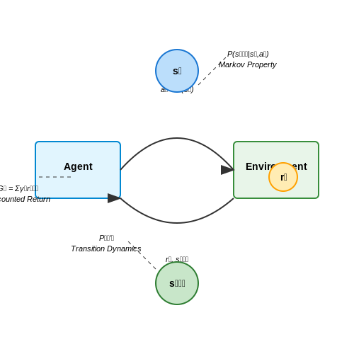
3.2 Markov Decision Processes (MDPs)
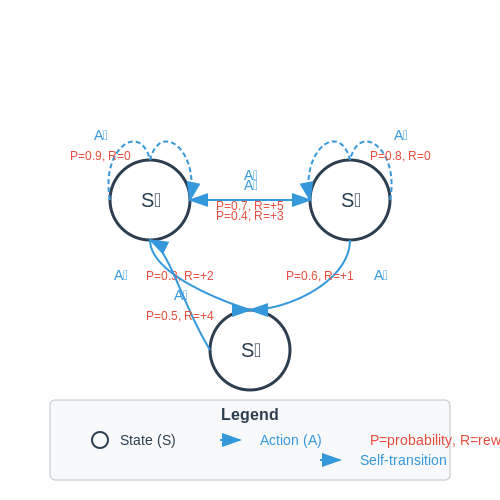
A Markov Decision Process (MDP) formalizes sequential decision-making in stochastic environments, serving as the foundational framework for reinforcement learning (RL). An MDP is defined by the tuple (S, A, P, R, γ), where:
- S: A finite set of states.
- A: A finite set of actions.
- P(s'|s, a): Transition dynamics specifying the probability of reaching state s' from state s after taking action a.
- R(s, a, s'): A reward function mapping transitions to scalar values.
- γ ∈ [0, 1]: A discount factor balancing immediate and future rewards.
Markov Property and State Transitions
The Markov property asserts that the future state st+1 depends only on the current state st and action at, independent of prior history. This is expressed as:
Bellman Equations
The value function Vπ(s), representing the expected cumulative reward under policy π, satisfies the Bellman expectation equation:
For an optimal policy π*, the Bellman optimality equation governs the optimal value function V*:
Policy Iteration and Value Iteration
Two classic dynamic programming methods solve MDPs:
- Policy Iteration: Alternates between policy evaluation (computing Vπ) and policy improvement (greedily updating π).
- Value Iteration: Directly iterates the Bellman optimality equation until convergence to V*.
Applications in OpenAI Gym
In OpenAI Gym, MDPs underpin environments like CartPole and MountainCar. For example, CartPole’s state space includes cart position and pole angle, while actions are discrete (left/right). The reward function encourages pole stability.
Exploration vs. Exploitation
The fundamental trade-off in reinforcement learning (RL) between exploration and exploitation governs how an agent balances gathering new information about the environment (exploration) versus leveraging existing knowledge to maximize rewards (exploitation). This trade-off is formalized mathematically and has profound implications for training agents in OpenAI Gym environments.
Mathematical Formulation
In the context of multi-armed bandits, the simplest RL setting, the exploration-exploitation dilemma is quantified using the regret metric. Regret measures the difference between the cumulative reward of the optimal policy and the agent's actual policy:
where T is the time horizon, μ* is the expected reward of the optimal action, and μat is the expected reward of the action taken at time t. Minimizing regret requires carefully balancing exploration and exploitation.
Strategies for Balancing Exploration and Exploitation
ε-Greedy Policy
The ε-greedy policy is a simple yet effective approach where the agent selects the action with the highest estimated value with probability 1-ε and a random action with probability ε:
where |A| is the number of possible actions. While easy to implement, ε-greedy can lead to suboptimal exploration in environments with sparse rewards.
Upper Confidence Bound (UCB)
UCB addresses ε-greedy's limitations by incorporating uncertainty estimates into action selection. The UCB1 algorithm selects actions based on:
where Nt(a) is the number of times action a has been selected by time t, and c is a hyperparameter controlling exploration. The second term ensures under-explored actions are prioritized.
Thompson Sampling
Thompson Sampling is a Bayesian approach where actions are selected proportionally to their probability of being optimal. For Bernoulli bandits, it maintains a Beta distribution over each action's success probability:
where αa and βa are the counts of successes and failures for action a. The agent samples from these distributions and selects the action with the highest sampled value.
Application in Deep Reinforcement Learning
In deep RL, exploration strategies must scale to high-dimensional state spaces. Common approaches include:
- Noise-based exploration: Adding noise to either the policy (e.g., parameter noise) or actions (e.g., Gaussian noise).
- Intrinsic motivation: Using curiosity-driven rewards based on prediction error or state novelty.
- Bootstrapped DQN: Maintaining multiple Q-value estimates and randomly sampling from them for action selection.
For example, in Proximal Policy Optimization (PPO), exploration is implicitly handled through the policy's entropy term:
where H is the entropy bonus encouraging stochastic policies.
Practical Considerations in OpenAI Gym
When implementing exploration strategies in OpenAI Gym, consider:
- The environment's reward structure (sparse vs. dense rewards).
- The dimensionality of the action space (discrete vs. continuous).
- Episodic vs. continuing tasks.
For continuous control tasks like Mujoco environments, adding correlated noise (e.g., Ornstein-Uhlenbeck process) to actions often yields better exploration than independent Gaussian noise.
4. Selecting an Appropriate Algorithm
4.1 Selecting an Appropriate Algorithm
Algorithm Selection Criteria
The choice of reinforcement learning (RL) algorithm in OpenAI Gym depends on the problem's characteristics, including the environment's dynamics, action space, observation space, and reward structure. Key considerations include:
- Discrete vs. Continuous Action Spaces: Q-learning and Deep Q-Networks (DQN) excel in discrete spaces, while policy gradient methods like Proximal Policy Optimization (PPO) or Trust Region Policy Optimization (TRPO) handle continuous actions.
- Episodic vs. Continuing Tasks: Monte Carlo methods suit episodic tasks with clear termination, while Temporal Difference (TD) methods like SARSA or TD(λ) adapt better to continuing tasks.
- Sample Efficiency: Model-based algorithms (e.g., Dyna-Q) require fewer environment interactions than model-free counterparts but demand accurate dynamics models.
Mathematical Foundations
The Bellman equation underpins most RL algorithms. For value-based methods like DQN, the optimal action-value function Q* satisfies:
where s is the state, a the action, r the reward, γ the discount factor, and 𝒫 the transition dynamics. Policy gradient methods directly optimize the policy πθ using the gradient:
where Ĵt is the advantage estimate, often computed using Generalized Advantage Estimation (GAE).
Advanced Algorithm Trade-offs
Soft Actor-Critic (SAC) introduces entropy regularization for exploration, with the objective:
where α controls exploration via entropy ℋ. For high-dimensional observations, Rainbow DQN combines six improvements (distributional RL, n-step returns) but increases computational overhead.
Implementation Considerations
When integrating algorithms with Gym's API, note that:
- On-policy algorithms (e.g., A2C, PPO) require fresh samples after each update, while off-policy methods (DDPG, SAC) reuse experience replay buffers.
- Gym's Box observation spaces may require normalization or convolutional neural networks (CNNs) for pixel inputs.
- Custom reward shaping often proves necessary to mitigate sparse rewards in environments like MountainCar or MontezumaRevenge.
Case Study: LunarLander-v2
For this continuous control task with 8D observations, PPO achieves stable convergence by:
- Clipping policy updates to avoid destructive large steps
- Using parallel actors for diversified exploration
- Normalizing advantages across mini-batches
The clipped surrogate objective is:
Implementing Q-Learning for Discrete Actions
Q-Learning is a model-free reinforcement learning algorithm that iteratively approximates the optimal action-value function Q*(s, a) by updating Q-values based on observed rewards and transitions. For discrete action spaces, the Q-table serves as a lookup table where each entry Q(s, a) represents the expected cumulative reward for taking action a in state s.
Mathematical Foundation
The Q-Learning update rule is derived from the Bellman equation, which decomposes the value of a state-action pair into the immediate reward and the discounted value of the next state:
Here, α is the learning rate (0 < α ≤ 1), and γ is the discount factor (0 ≤ γ ≤ 1). The term rt+1 + γ maxa Q(st+1, a) is the TD target, representing the updated estimate of the optimal Q-value.
Algorithm Implementation Steps
- Initialize Q-table: Create a matrix of zeros with dimensions (num_states × num_actions).
- Select action: Use an exploration strategy (e.g., ε-greedy) to balance exploration and exploitation.
- Execute action: Observe the next state s' and reward r.
- Update Q-value: Apply the Bellman update to adjust the Q-table entry for (s, a).
- Repeat: Iterate until convergence or a stopping criterion is met.
Practical Considerations
In OpenAI Gym, discrete action spaces (e.g., in CartPole or FrozenLake) require discretizing continuous state variables if necessary. For high-dimensional state spaces, consider function approximation (e.g., Deep Q-Networks) instead of tabular Q-Learning.
Example: Q-Learning for FrozenLake
import numpy as np
import gym

env = gym.make('FrozenLake-v1', is_slippery=False)
Q = np.zeros((env.observation_space.n, env.action_space.n))

alpha = 0.1
gamma = 0.99
epsilon = 0.1

for episode in range(10000):
   state = env.reset()
   done = False
   while not done:
      if np.random.rand() < epsilon:
         action = env.action_space.sample()
      else:
         action = np.argmax(Q[state, :])
      next_state, reward, done, _ = env.step(action)
      Q[state, action] += alpha * (reward + gamma * np.max(Q[next_state, :]) - Q[state, action])
      state = next_state
Convergence and Optimality
Under the Robbins-Monro conditions for stochastic approximation, Q-Learning converges to the optimal Q-function if:
- All state-action pairs are visited infinitely often.
- The learning rate α satisfies ∑t αt = ∞ and ∑t αt2 < ∞.
In practice, ε-greedy exploration and decaying learning rates are used to approximate these conditions.
Deep Q-Networks (DQN) for Complex Environments
Deep Q-Networks (DQN) extend traditional Q-learning by approximating the Q-function using a deep neural network, enabling the handling of high-dimensional state spaces. The core idea is to replace the tabular Q-table with a function approximator, allowing generalization across states. The loss function for training the network is derived from the Bellman equation:
Here, θ represents the network parameters, θ⁻ denotes the target network parameters (fixed for stability), and D is the experience replay buffer. The target network is periodically updated to match the current network, reducing the risk of divergence.
Experience Replay and Target Networks
Experience replay stores transitions (s, a, r, s') in a buffer, allowing the agent to learn from past experiences. This breaks temporal correlations and improves sample efficiency. The target network, a delayed copy of the main network, provides stable Q-value targets during training. The update rule for the target network is:
where τ is a small interpolation factor (e.g., 0.001). This soft update ensures gradual changes to the target network, preventing abrupt shifts in Q-value estimates.
Architectural Choices for DQN
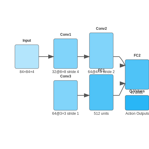
For image-based environments (e.g., Atari games), the network typically consists of convolutional layers followed by fully connected layers:
- Input: Preprocessed frame stack (84×84×4 grayscale images).
- Convolutional Layers: Three layers with ReLU activation (32, 64, and 64 filters, kernel sizes 8×8, 4×4, and 3×3, strides 4, 2, and 1).
- Fully Connected Layers: Two layers (512 and N units, where N is the number of actions).
For non-visual tasks, the architecture may use multilayer perceptrons (MLPs) with batch normalization and dropout for regularization.
Double DQN and Prioritized Experience Replay
Double DQN addresses overestimation bias by decoupling action selection and evaluation:
Prioritized experience replay assigns higher sampling probability to transitions with high temporal-difference (TD) error, accelerating learning. The probability P(i) for sampling transition i is:
where p_i is the priority (often proportional to TD error) and α controls the prioritization strength.
Practical Implementation in OpenAI Gym
The following code snippet demonstrates a DQN implementation for the CartPole environment using PyTorch:
import torch
import torch.nn as nn
import torch.optim as optim
import numpy as np
from collections import deque
import random

class DQN(nn.Module):
    def __init__(self, state_dim, action_dim):
        super(DQN, self).__init__()
        self.fc1 = nn.Linear(state_dim, 64)
        self.fc2 = nn.Linear(64, 64)
        self.fc3 = nn.Linear(64, action_dim)

    def forward(self, x):
        x = torch.relu(self.fc1(x))
        x = torch.relu(self.fc2(x))
        return self.fc3(x)

class ReplayBuffer:
    def __init__(self, capacity):
        self.buffer = deque(maxlen=capacity)

    def push(self, state, action, reward, next_state, done):
        self.buffer.append((state, action, reward, next_state, done))

    def sample(self, batch_size):
        return random.sample(self.buffer, batch_size)

    def __len__(self):
        return len(self.buffer)
Key hyperparameters include a replay buffer size of 10⁵, batch size of 64, discount factor γ=0.99, and an ε-greedy exploration schedule decaying from 1.0 to 0.01 over 10,000 steps.
4.4 Policy Gradient Methods
Policy gradient methods optimize the policy directly by adjusting its parameters θ to maximize expected reward. Unlike value-based methods, which learn a value function and derive a policy indirectly, policy gradients parameterize the policy πθ(a|s) and update θ using gradient ascent on the performance measure J(θ).
Policy Gradient Theorem
The foundation of policy gradient methods lies in the Policy Gradient Theorem, which provides an analytical expression for the gradient of the performance measure with respect to the policy parameters:
Here, dπ is the state distribution under policy πθ, and Qπ(s,a) is the state-action value function. This gradient can be estimated via Monte Carlo sampling, enabling stochastic gradient ascent.
REINFORCE Algorithm
The REINFORCE algorithm, a Monte Carlo policy gradient method, approximates the gradient using complete episode trajectories:
where Gt is the return from time step t. The policy parameters are updated as:
Despite its simplicity, REINFORCE suffers from high variance due to relying on full Monte Carlo returns. Variance reduction techniques, such as baselines, are often employed.
Advantage Actor-Critic (A2C)
A2C reduces variance by combining policy gradients with a learned value function. The gradient is computed using the advantage function Aπ(s,a) = Qπ(s,a) − Vπ(s):
The critic network estimates Vπ(s), while the actor updates the policy using the advantage. This approach stabilizes training by decoupling policy and value updates.
Proximal Policy Optimization (PPO)
PPO improves stability by constraining policy updates to prevent large deviations. The objective function includes a clipped surrogate advantage:
where rt(θ) = πθ(at|st) / πθold(at|st) is the probability ratio, and ϵ is a hyperparameter controlling the clipping range.
Practical Implementation in OpenAI Gym
Below is an example of implementing REINFORCE in OpenAI Gym using PyTorch:
import torch
import torch.nn as nn
import torch.optim as optim
import gym

class PolicyNetwork(nn.Module):
    def __init__(self, state_dim, action_dim):
        super().__init__()
        self.fc = nn.Sequential(
            nn.Linear(state_dim, 64),
            nn.ReLU(),
            nn.Linear(64, action_dim),
            nn.Softmax(dim=-1)
        )

    def forward(self, state):
        return self.fc(state)

env = gym.make("CartPole-v1")
policy = PolicyNetwork(env.observation_space.shape[0], env.action_space.n)
optimizer = optim.Adam(policy.parameters(), lr=0.01)

def reinforce(episodes=1000, gamma=0.99):
    for _ in range(episodes):
        state = env.reset()
        log_probs = []
        rewards = []

        while True:
            state = torch.FloatTensor(state)
            action_probs = policy(state)
            action = torch.multinomial(action_probs, 1).item()

            next_state, reward, done, _ = env.step(action)
            log_probs.append(torch.log(action_probs[action]))
            rewards.append(reward)
            state = next_state

            if done:
                break

        # Compute discounted returns
        returns = []
        G = 0
        for r in reversed(rewards):
            G = r + gamma * G
            returns.insert(0, G)

        # Update policy
        policy_loss = []
        for log_prob, G in zip(log_probs, returns):
            policy_loss.append(-log_prob * G)

        optimizer.zero_grad()
        loss = torch.stack(policy_loss).sum()
        loss.backward()
        optimizer.step()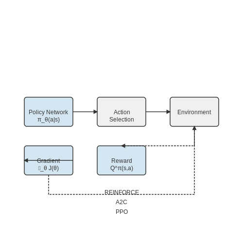
4.5 Monitoring and Evaluating Agent Performance
Key Performance Metrics
Effective evaluation of reinforcement learning agents requires tracking multiple metrics beyond cumulative reward. The episodic return \( G_t = \sum_{k=0}^{T} \gamma^k r_{t+k} \) provides a discounted sum of rewards, but variance reduction techniques like reward normalization or advantage estimation are often necessary for stable training. For continuous control tasks, domain-specific metrics such as:
- Average action smoothness \( \frac{1}{T}\sum_{t=1}^{T} ||a_t - a_{t-1}||_2 \)
- Energy consumption \( \sum_{t=1}^{T} a_t^T R a_t \) (where \( R \) is a cost matrix)
- Task completion time
provide additional insight into agent behavior.
Statistical Significance Testing
When comparing algorithms, Welch's t-test accounts for unequal variances between runs:
where \( \bar{X} \) denotes sample means and \( s^2 \) sample variances. For non-normal distributions, the Mann-Whitney U test is preferred. OpenAI Gym's monitor wrapper automatically logs these statistics at configurable intervals.
Visualization Techniques
TensorBoard integration provides real-time plotting of:
- Smoothed reward curves with exponential moving averages
- Value function heatmaps for discrete state spaces
- Policy entropy \( \mathcal{H}(\pi(\cdot|s)) = -\sum_a \pi(a|s)\log\pi(a|s) \)
For Atari environments, frame stacking with overlayed action distributions reveals temporal decision patterns.
Diagnosing Training Failures
Common failure modes exhibit distinct signatures:
| Failure Mode | Diagnostic Indicator |
|---|---|
| Catastrophic forgetting | Spikes in TD error \( \delta_t = r_t + \gamma V(s_{t+1}) - V(s_t) \) |
| Overestimation bias | Q-values diverge from Monte Carlo returns |
| Exploration collapse | Policy entropy drops below \( 0.1 \times \log(|\mathcal{A}|) \) |
Benchmarking Against Baselines
The gym.benchmark registry provides reference implementations with pretrained weights. For custom tasks, implement:
def compute_relative_improvement(agent_perf, baseline_perf):
    return (agent_perf - baseline_perf) / (max_perf - baseline_perf)
where max_perf is the theoretical maximum return. For stochastic environments, use at least 100 episodes per evaluation.
5. Hyperparameter Tuning for Better Performance
5.1 Hyperparameter Tuning for Better Performance
Hyperparameter tuning is critical for optimizing reinforcement learning (RL) agents in OpenAI Gym. Unlike model parameters learned during training, hyperparameters are set before training begins and govern the learning process itself. Key hyperparameters include learning rate, discount factor (γ), exploration rate (ε), and batch size, each influencing convergence speed and final performance.
Learning Rate (α)
The learning rate controls how much the agent updates its policy or value function in response to new data. A high learning rate may cause instability, while a low rate leads to slow convergence. The optimal learning rate often follows the Robbins-Monro conditions:
In practice, adaptive methods like Adam or RMSprop dynamically adjust α during training. For Q-learning, a common starting range is α ∈ [0.001, 0.1], validated through grid search or Bayesian optimization.
Discount Factor (γ)
γ determines the present value of future rewards, with γ = 0 making the agent myopic and γ ≈ 1 encouraging long-term planning. The choice depends on the environment's horizon:
where H is the effective horizon. For episodic tasks like CartPole (H ≈ 200), γ = 0.99 is typical, while continuous tasks may require γ ≥ 0.999.
Exploration-Exploitation Trade-off
ε-greedy policies balance exploration and exploitation by decaying ε over time. A common schedule is:
where λ controls the decay rate. Alternative strategies like Boltzmann exploration or Upper Confidence Bound (UCB) may outperform ε-greedy in sparse-reward environments.
Batch Size and Replay Buffer
For deep RL (e.g., DQN), batch size affects gradient estimation quality. Larger batches reduce variance but increase computational cost. The replay buffer size should be large enough to decorrelate samples but not so large as to stall learning. Empirical studies suggest:
where Nparams is the number of network parameters. For a DQN with ~1M parameters, B = 32–128 is typical.
Automated Tuning Methods
Manual tuning is often suboptimal. Advanced techniques include:
- Bayesian Optimization: Models the performance landscape using Gaussian processes to guide sampling.
- Population-Based Training (PBT): Simultaneously trains and mutates hyperparameters across a population of agents.
- Meta-Gradient RL: Learns hyperparameter adaptation policies end-to-end.
Tools like Optuna or Ray Tune integrate with OpenAI Gym for distributed hyperparameter search. Below is an example of implementing Bayesian optimization for a DQN agent:
import optuna
from stable_baselines3 import DQN

def objective(trial):
    lr = trial.suggest_float("lr", 1e-5, 1e-2, log=True)
    gamma = trial.suggest_float("gamma", 0.9, 0.9999)
    batch_size = trial.suggest_categorical("batch_size", [32, 64, 128])

    model = DQN(
        "MlpPolicy",
        "CartPole-v1",
        learning_rate=lr,
        gamma=gamma,
        batch_size=batch_size,
        verbose=0
    )
    model.learn(total_timesteps=10000)
    mean_reward = evaluate_policy(model, n_eval_episodes=10)
    return mean_reward

study = optuna.create_study(direction="maximize")
study.optimize(objective, n_trials=50)
5.2 Using Custom Environments
OpenAI Gym's predefined environments are useful for benchmarking, but real-world applications often require custom environments tailored to specific problems. Creating a custom Gym environment involves subclassing gym.Env and implementing key methods: __init__, step, reset, and render. The environment must also define action_space and observation_space using Gym's Space API.
Environment Structure
A custom environment must adhere to the following structure:
import gym
from gym import spaces
import numpy as np

class CustomEnv(gym.Env):
    def __init__(self):
        super(CustomEnv, self).__init__()
        self.action_space = spaces.Discrete(3)  # Example: 3 discrete actions
        self.observation_space = spaces.Box(low=0, high=1, shape=(4,), dtype=np.float32)

    def step(self, action):
        # Execute action, return (observation, reward, done, info)
        pass

    def reset(self):
        # Reset environment to initial state
        pass

    def render(self, mode='human'):
        # Optional: Visualize the environment
        pass
Defining Observation and Action Spaces
The observation_space and action_space define the structure of valid inputs and outputs. Gym provides several space types:
- Discrete: A finite set of actions (e.g.,
spaces.Discrete(4)for 4 possible actions). - Box: A continuous n-dimensional space (e.g.,
spaces.Box(low=-1, high=1, shape=(3,))for a 3D vector). - MultiDiscrete: A set of discrete actions with independent ranges.
- Dict: A dictionary of simpler spaces for complex observations.
Reward Engineering
The step method must return a reward signal that guides the agent toward desired behavior. Poorly shaped rewards can lead to suboptimal policies. For example, sparse rewards (only given at task completion) make learning difficult, while dense rewards (frequent feedback) accelerate training but may introduce unintended biases.
where wi are weights and fi are reward components (e.g., distance to goal, time penalty).
Registering Custom Environments
To integrate a custom environment with Gym's API, register it using gym.register:
from gym.envs.registration import register

register(
    id='CustomEnv-v0',
    entry_point='custom_env:CustomEnv',
    max_episode_steps=500,
)
After registration, the environment can be created using gym.make('CustomEnv-v0').
Debugging and Validation
Before training, validate the environment using random actions to ensure correct behavior:
env = gym.make('CustomEnv-v0')
obs = env.reset()
for _ in range(1000):
    action = env.action_space.sample()
    obs, reward, done, info = env.step(action)
    if done:
        obs = env.reset()
Common issues include incorrect observation shapes, invalid actions, or improperly defined spaces. Use Gym's built-in checks via from gym.utils.env_checker import check_env; check_env(env).
Advanced Customization
For complex environments, consider:
- Parallel Execution: Use
VectorEnvfor batched simulations. - Wrappers: Modify existing environments using wrappers (e.g.,
TimeLimit,Monitor). - Stochastic Dynamics: Introduce randomness in state transitions for robustness.
5.3 Parallel Training with Vectorized Environments
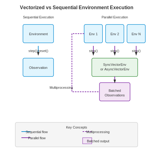
Vectorized environments enable simultaneous execution of multiple independent environments, drastically improving sample efficiency and training speed. Unlike sequential training, where agents interact with one environment at a time, vectorization leverages parallelization to collect batches of experiences in a single step. This approach is particularly effective in reinforcement learning (RL), where sample efficiency is critical.
Architecture of Vectorized Environments
A vectorized environment wraps multiple instances of a base environment, executing their step and reset functions in parallel. The observations, rewards, and termination flags are returned as stacked arrays, allowing batched processing. OpenAI Gym's SyncVectorEnv and AsyncVectorEnv are two primary implementations:
- SyncVectorEnv: Executes environments sequentially but returns batched outputs. Suitable for lightweight environments where parallel overhead outweighs benefits.
- AsyncVectorEnv: Uses multiprocessing for true parallelism, ideal for CPU-bound tasks like physics simulations.
Mathematical Efficiency Gains
Let N be the number of environments, T the time per environment step, and O the overhead of parallelization. The speedup factor S is given by:
For AsyncVectorEnv, O is negligible when N is large, approaching linear speedup. Empirical studies show a 5–10× improvement for N = 16 in Atari environments.
Implementation in OpenAI Gym
The following example demonstrates vectorized environment creation using gym.vector.make:
import gym
from gym.vector import SyncVectorEnv

def make_env(env_id):
    def _thunk():
        env = gym.make(env_id)
        return env
    return _thunk

envs = SyncVectorEnv([make_env("CartPole-v1") for _ in range(8)])
obs = envs.reset()  # Shape: (8, 4)
Challenges and Mitigations
Vectorization introduces two key challenges:
- Non-uniform episode lengths: Environments may terminate at different times. Solutions include auto-resetting terminated environments and masking their contributions to gradients.
- Memory overhead: Storing observations for all environments requires O(N) memory. Gradient checkpointing or mixed-precision training can alleviate this.
Case Study: Proximal Policy Optimization (PPO)
PPO benefits significantly from vectorization. With N = 32 environments, a single policy update can utilize 32× more samples than sequential training, reducing wall-clock time by 85% in MuJoCo benchmarks. The policy gradient loss for a vectorized batch is:
6. Handling Sparse Rewards
6.1 Handling Sparse Rewards
Sparse rewards present a significant challenge in reinforcement learning (RL), where the agent receives infrequent or delayed feedback. This scenario is common in real-world tasks such as robotic manipulation, autonomous navigation, or game-solving, where meaningful rewards are rare relative to the state-action space. Without dense reward signals, traditional RL algorithms struggle with exploration and credit assignment.
Credit Assignment in Sparse Reward Environments
The temporal credit assignment problem arises when an agent must associate a reward with a sequence of actions leading to it. In sparse reward settings, this becomes exponentially harder due to the lack of intermediate feedback. Consider an episodic task where the agent receives a reward only upon success. The probability of stumbling upon the correct action sequence by random exploration is:
where at* denotes the optimal action at time t. For large T, this probability decays rapidly, making learning intractable.
Intrinsic Motivation and Exploration
To mitigate this, intrinsic motivation mechanisms encourage exploration by rewarding the agent for discovering novel states or reducing uncertainty. Two prominent approaches are:
- Count-based exploration: The agent maintains a state visitation count N(s) and receives an intrinsic reward inversely proportional to N(s):
where β scales the exploration bonus.
- Prediction error-based exploration: Models like Random Network Distillation (RND) use the error of a neural network predicting features of unseen states as an intrinsic reward.
Hindsight Experience Replay (HER)
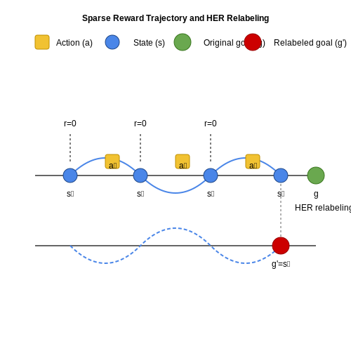
HER addresses sparse rewards by relabeling failed trajectories with artificial goals. For a trajectory τ = (s0, a0, ..., sT) that did not achieve the original goal g, HER stores transitions with modified goals g' = sT and rewards indicating whether g' was achieved. The Q-learning update becomes:
Reward Shaping and Curriculum Learning
Reward shaping introduces auxiliary rewards to guide the agent toward the true objective. A well-designed shaping function F(s, a, s') must satisfy potential-based criteria to preserve optimal policies:
where Φ is a potential function. Curriculum learning progressively increases task difficulty, starting with dense rewards and gradually transitioning to sparser ones.
Case Study: Montezuma’s Revenge
This Atari game exemplifies sparse rewards, where the agent must complete a sequence of precise actions to obtain the first reward. State-of-the-art methods combining intrinsic motivation, hierarchical RL, and imitation learning have achieved success. For instance, an agent trained with RND and HER can learn to navigate early rooms by maximizing exploration bonuses before encountering extrinsic rewards.
6.2 Addressing Non-Stationarity
Non-stationarity in reinforcement learning (RL) arises when the environment's dynamics or reward distribution change over time, violating the Markov assumption. This poses a significant challenge for training agents in OpenAI Gym, as traditional RL algorithms assume stationary environments. Non-stationarity can emerge from multiple sources, including adversarial opponents, evolving system dynamics, or shifting reward functions.
Sources of Non-Stationarity
In multi-agent RL, non-stationarity is intrinsic because other agents adapt their policies concurrently, altering the environment from a single agent's perspective. Mathematically, if agent i interacts with agent j, the transition dynamics P(s'|s, ai, aj) and reward function R(s, ai, aj) depend on both agents' actions. As agent j updates its policy πj, the environment becomes non-stationary for agent i:
Similarly, in single-agent settings, non-stationarity may arise from environment drift, such as mechanical wear in robotics or concept drift in recommendation systems.
Empirical Strategies for Mitigation
Several empirically validated approaches address non-stationarity:
- Experience Replay with Importance Sampling: Prioritized experience replay buffers store past transitions, allowing agents to revisit earlier environment dynamics. Importance weights correct for distributional shifts when sampling from the buffer.
- Meta-Learning Frameworks: Algorithms like MAML (Model-Agnostic Meta-Learning) train agents to adapt quickly to new dynamics by optimizing for performance across a distribution of tasks.
- Adversarial Training: In multi-agent settings, self-play or population-based training exposes agents to diverse opponents, improving robustness to policy shifts.
Theoretical Foundations: Convergence Guarantees
For tabular Q-learning, convergence proofs assume stationary environments. Non-stationarity breaks these guarantees, but theoretical workarounds exist. One approach uses decaying learning rates αt that satisfy the Robbins-Monro conditions:
This ensures sufficient exploration while gradually reducing the impact of outdated Q-values. For continuous state spaces, Gradient Temporal Difference (GTD) methods provide stability under non-stationarity by minimizing the mean-squared projected Bellman error.
Implementation in OpenAI Gym
To handle non-stationarity in OpenAI Gym, wrap the environment to inject dynamics shifts or opponent policy updates. Below is a Python example using a custom wrapper that periodically alters transition probabilities:
import gym
from gym import spaces
import numpy as np

class NonStationaryWrapper(gym.Wrapper):
    def __init__(self, env, change_interval=1000):
        super().__init__(env)
        self.change_interval = change_interval
        self.step_count = 0
        self.current_dynamics = self.sample_dynamics()

    def sample_dynamics(self):
        # Randomly perturb transition probabilities
        return np.random.uniform(0.8, 1.2, size=self.env.observation_space.shape)

    def step(self, action):
        self.step_count += 1
        if self.step_count % self.change_interval == 0:
            self.current_dynamics = self.sample_dynamics()

        obs, reward, done, info = self.env.step(action)
        modified_obs = obs * self.current_dynamics  # Apply dynamics shift
        return modified_obs, reward, done, info
Case Study: Non-Stationarity in Atari Games
In Pong, a self-play RL agent faces non-stationarity as the opponent's policy improves. A practical solution combines:
- Population-Based Training (PBT): Maintain a pool of agents with diverse strategies, periodically replacing weak opponents.
- Proximal Policy Optimization (PPO): The clipped objective function prevents drastic policy updates, reducing sensitivity to opponent changes.
where rt(θ) is the probability ratio between new and old policies, and Ât is the advantage estimate.
6.3 Debugging Training Failures
Diagnosing Vanishing or Exploding Gradients
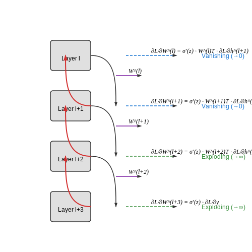
Training failures in reinforcement learning (RL) often stem from unstable gradients, particularly in deep neural networks. The gradient magnitude can vanish or explode exponentially across layers, impeding convergence. For a network with L layers, the gradient ∂L/∂W(l) for layer l is:
where σ' is the derivative of the activation function and z(i) are pre-activations. If the product term’s eigenvalues deviate from 1, gradients vanish (→0) or explode (→∞). Mitigation strategies include:
- Gradient clipping: Enforce a maximum norm for gradients, e.g., ||g|| ≤ c.
- Weight initialization: Use He or Xavier initialization to preserve variance across layers.
- Batch normalization: Normalize layer inputs to stabilize activations.
Reward Design and Sparse Rewards
Poor reward shaping leads to uninformative gradients. For sparse rewards, the agent receives feedback only after lengthy trajectories, causing high variance in policy updates. Consider:
- Dense reward proxies: Augment sparse rewards with auxiliary objectives (e.g., curiosity-driven exploration).
- Reward scaling: Normalize rewards to a consistent range (e.g., [-1, 1]) to prevent magnitude mismatches.
- Advantage estimation: Use Generalized Advantage Estimation (GAE) to reduce variance in policy gradients:
Hyperparameter Sensitivity
RL algorithms are highly sensitive to hyperparameters like learning rate (α), discount factor (γ), and entropy coefficient. For example, a suboptimal α may cause:
- Overshooting: Large α leads to divergent weight updates.
- Stagnation: Small α results in impractically slow convergence.
Use automated tools like Optuna or Ray Tune for hyperparameter search, or adopt adaptive optimizers (e.g., Adam with learning rate warmup).
Debugging Tools and Techniques
Instrument training with the following diagnostics:
- Gradient histograms: Visualize layer-wise gradient distributions (e.g., TensorBoard).
- Value function checks: Monitor the critic’s predictions to detect over/underestimation bias.
- Exploration metrics: Track state visitation entropy to identify premature convergence.
# Example: Logging gradients in PyTorch
from torch.utils.tensorboard import SummaryWriter

writer = SummaryWriter()
for name, param in model.named_parameters():
    if param.grad is not None:
        writer.add_histogram(f"{name}_grad", param.grad, global_step)
Environment and Implementation Bugs
Subtle bugs in environment dynamics or agent logic can manifest as training failures. Common pitfalls include:
- Non-stationarity: If the environment changes during training (e.g., due to random seeds), the agent fails to generalize.
- Incorrect action spaces: Mismatched dimensions between policy outputs and environment actions.
- Observation preprocessing: Missing normalization or clipping of inputs alters the effective state space.
7. Essential Research Papers
7.1 Essential Research Papers
- PDF Training reinforcement learning model with custom OpenAI gym for IIoT ... — 2.4.2 Developing an OpenAI Gym-compatible framework and simulation environment for testing Deep Reinforcement Learning agents solving the Ambulance Location Problem ..... 15 2.4.3 Reinforcement learning for adaptive order dispatching in the
- Integrating OpenAI Gym and CloudSim Plus: A simulation environment for ... — In this study, we create two environments: the targeted environment (using CloudSim Plus [13]) and the agent's training environment (using OpenAI Gym [46]). The interaction between these environments has been illustrated as in Fig. 2. They are integrated, with the targeted environment simulating the cloud scaling process in advance to provide ...
- PDF HDDLGym: A Tool for Studying Multi-Agent Hierarchical Problems Defined ... — ing multi-agent scenarios and enabling collaborative plan-ning among agents. This paper provides an overview of HD-DLGym's design and implementation, highlighting the chal-lenges and design choices involved in integrating HDDL with the Gym interface and applying RL policies to hierarchical planning. We also provide detailed instructions and ...
- Practical Reinforcement Learning: Develop Self-evolving, Intelligent ... — OpenAI Gym OpenAI is a non-profit AI research company. OpenAI Gym is a toolkit for developing and comparing reinforcement learning algorithms. The gym open source library is a collection of test problems— environments—that can be used to work out our reinforcement learning algorithms.
- PDF AA228/CS238 FINAL PROJECT PAPER, DECEMBER 2019 1 Solving The Lunar ... — Abstract—Reinforcement Learning (RL) is an area of machine learning concerned with enabling an agent to navigate an environment with uncertainty in order to maximize some notion of cumulative long-term reward. In this paper, we implement and analyze two different RL techniques, Sarsa and Deep Q-Learning on OpenAI Gym's LunarLander-v2 ...
- gym/README.rst at 31be35ecd460f670f0c4b653a14c9996b7facc6c · openai/gym ... — OpenAI Gym is a toolkit for developing and comparing reinforcement learning algorithms. This is the gym open-source library, which gives you access to a standardized set of environments.. See What's New section below. gym makes no assumptions about the structure of your agent, and is compatible with any numerical computation library, such as TensorFlow or Theano.
- ns-3 meets OpenAI Gym: The Playground for Machine Learning in ... — This paper presents the ns3-gym - the first framework for RL research in networking. It is based on OpenAI Gym, a toolkit for RL research and ns-3 network simulator.
- (PDF) Integrating Openai Gym and Cloudsim Plus: A Simulation ... — By leveraging the strengths of both Python-based OpenAI Gym and Java-based CloudSim Plus, the simulation environment o ff ers a flexible and extensible platform for DRL agent training. The ...
- Training an Agent to play Pong using Reinforcement Learning — 3. Implementation of the Solution. To implement the environment we use the OpenAI Gym tools. We will use the TF-Agents python library from Google to implement the agent.Because we have discrete actions we will use the Deep Q Network (DQN) network as a function approximator for the agent.. This implementation allows the agent to give simple categorical commands to its own paddle.
- GitHub - sfujim/TD3: Author's PyTorch implementation of TD3 for OpenAI ... — The first evaluation is the randomly initialized policy network (unused in the paper). Evaluations are peformed every 5000 time steps, over a total of 1 million time steps. Numerical results can be found in the paper, or from the learning curves. Video of the learned agent can be found here.
7.2 Recommended Books and Courses
- PDF Electrical Engineering Principles And Applications Read Online - old ... — Read Online Cloud ComputingAbstract AlgebraAn Introduction to Statistical LearningUniversal Design for Web ApplicationsIodine Chemistry and ApplicationsMastering ShinyJavaScript Web ApplicationsEngineering Production-grade Shiny AppsEconomicsAbstract Algebra with ApplicationsScience and Application of High-Intensity Interval TrainingWeb Technologies: Concepts, Methodologies, Tools, and ...
- Awesome Machine Learning - GitHub — PyBroker - Algorithmic Trading with Machine Learning. Frouros: Frouros is an open source Python library for drift detection in machine learning systems. CometML: The best-in-class MLOps platform with experiment tracking, model production monitoring, a model registry, and data lineage from training straight through to production.
- Practical Reinforcement Learning: Develop Self-evolving, Intelligent ... — Practical Reinforcement Learning: Develop Self-evolving, Intelligent Agents With Openai Gym, Python And Java [PDF] [2t7us3n1ng7g]. ...
- Integrating OpenAI Gym and CloudSim Plus: A simulation environment for ... — The proposed simulator specifically focuses on the case study of energy-driven cloud scaling. By leveraging the strengths of both Python-based OpenAI Gym and Java-based CloudSim Plus, the simulation environment offers a flexible and extensible platform for DRL-Agent training.
- All jobs from Hacker News 'Who is hiring? (December 2021)' post | HNHIRING — We are West Coast based, but have remote employees all over the United States. WELL has been named No. 10 on the 2021 Forbes America's Best Startup Employers list. In 2020, WELL Health was named among the Best Places to Work by Modern Healthcare and ranked #170 on the Inc. 5000 list of fastest growing private companies.
- New Era of Artificial Intelligence in Education: - ProQuest — Artificial intelligence (AI) has quickly established itself as a transformative force in a wide range of industries, including education. The development of AI has resulted in an array of advancements and innovations that have impacted many facets of human life. As a fundamental component to societal evolution and individual development, education has had significant benefits from AI ...
- The Best OpenAI Books of All Time - BookAuthority — The best openai books recommended by Luca Zavarella and Andy McMahon, such as Exploring GPT-3, HANDBOOK OF CHATGPT and OpenAI API Cookbook.
- Ask HN: What are you working on? (April 2025) - Hacker News — Colibri is as much a tool I personally want to use, as it is a study in small-audience user interfaces, and the quest to build the perfect book catalog schema. I'm looking for fellow book-loving people to work on Colibri, to create the best personal digital library possible.
- Newsletter — South Africa's #1 startup newsletter featuring big trends and who is capitalising on them and a builder's corner, featuring practical startup building tips.
- DOC ΕΛΛΗΝΙΚΗ ΔΗΜΟΚΡΑΤΙΑ — 2.d. Any other family member of an EU national, if s/he is supported by the EU national or living under his roof in the country of origin or if serious health reasons make it necessary for the EU national to take care of him or her, or maintains the EU national with a right of residence: 143
7.3 Community Resources and Forums
- Reinforcement Learning with OpenAI Gym: A Practical Guide — Getting Started with OpenAI Gym. OpenAI Gym offers a powerful toolkit for developing and testing reinforcement learning algorithms. To get started with this versatile framework, follow these essential steps. First, install the library. Open your terminal and execute: pip install gym. This command will fetch and install the core Gym library.
- OpenAI Gym Beta — We want OpenAI Gym to be a community effort from the beginning. We've starting working with partners to put together resources around OpenAI Gym: NVIDIA (opens in a new window): technical Q&A (opens in a new window) with John. Nervana (opens in a new window): implementation of a DQN OpenAI Gym agent (opens in a new window).
- Intro to Reinforcement Learning | OpenAI Gym, RLlib & Google Colab — Link Training an Agent. In reinforcement learning, the goal of the agent is to produce smarter and smarter actions over time. It does so with a policy. In deep reinforcement learning, this policy is represented with a neural network. Let's first interact with the RL gym environment without a neural network or machine learning algorithm of any kind.
- gym/README.rst at 31be35ecd460f670f0c4b653a14c9996b7facc6c · openai/gym ... — OpenAI Gym is a toolkit for developing and comparing reinforcement learning algorithms. This is the gym open-source library, which gives you access to a standardized set of environments.. See What's New section below. gym makes no assumptions about the structure of your agent, and is compatible with any numerical computation library, such as TensorFlow or Theano.
- Get Started with OpenAI Gym API - toolify.ai — OpenAI Gym's API provides a unified interface for interacting with a wide range of environments for reinforcement learning. Through the use of Gym environments, wrappers, and monitors, users can easily experiment, extend functionality, and monitor their agent's performance. Resources. OpenAI Gym; OpenAI Gym GitHub Repository; Highlights
- Tutorials - Gym Documentation — Tutorials. Getting Started With OpenAI Gym: The Basic Building Blocks; Reinforcement Q-Learning from Scratch in Python with OpenAI Gym; Tutorial: An Introduction to Reinforcement Learning Using OpenAI Gym
- Can I build AI agents with OpenAI Gym? - milvus.io — OpenAI Gym integrates with libraries like TensorFlow or PyTorch for this purpose, allowing you to train agents using gradient-based optimization. Practical implementation involves setting up a training loop where the agent interacts with the environment over many episodes.
- GitHub - openai/gym: A toolkit for developing and comparing ... — Gym is an open source Python library for developing and comparing reinforcement learning algorithms by providing a standard API to communicate between learning algorithms and environments, as well as a standard set of environments compliant with that API.
- Getting Started With OpenAI Gym: The Basic Building Blocks — pip install -U gym Environments. The fundamental building block of OpenAI Gym is the Env class. It is a Python class that basically implements a simulator that runs the environment you want to train your agent in. Open AI Gym comes packed with a lot of environments, such as one where you can move a car up a hill, balance a swinging pendulum, score well on Atari games, etc. Gym also provides ...
- A Gentle Introduction to OpenAI Gym | intro_to_gym - Weights & Biases — Here's an example using the Frozen Lake environment from Gym. Our agent is an elf and our environment is the lake. It's frozen, so it's slippery. If our agent (a friendly elf) chooses to go left, there's a one in five chance he'll slip and move diagonally instead. Here, t he slipperiness determines where the agent will end up. In ...