Self-Auditing AI Chains with Modular Monitoring
1. Defining AI Chains and Modular Components
1.1 Defining AI Chains and Modular Components
AI chains represent a paradigm shift in complex system design, where a sequence of interconnected machine learning models or algorithmic components operate in a coordinated pipeline to achieve a composite objective. Unlike monolithic architectures, these chains decompose tasks into specialized modules, each responsible for a distinct subtask while maintaining interoperability through well-defined interfaces.
Formal Definition of AI Chains
An AI chain C can be formally represented as a directed acyclic graph (DAG) where nodes correspond to processing modules and edges define data dependencies:
where:
- M = {m1, m2, ..., mn} is the set of n modular components
- E ⊆ M × M defines the execution dependencies between modules
The information flow through the chain follows topological ordering, with each module mi processing inputs Ii to produce outputs Oi according to its internal function fi:
Characteristics of Modular Components
Effective modularization in AI chains requires components to exhibit three fundamental properties:
- Functional Encapsulation: Each module maintains a single responsibility principle with clearly defined input/output contracts
- Interface Standardization: Communication between modules occurs through versioned API contracts or standardized data formats
- Independent Deployability: Modules can be updated, replaced, or scaled without requiring changes to adjacent components
Implementation Considerations
In practice, modular components often manifest as:
- Containerized microservices with gRPC or REST interfaces
- Parameterized machine learning models with standardized input tensors
- Deterministic algorithmic components with versioned I/O schemas
The computational graph for a text processing chain might include:
Monitoring Implications
Modular architecture enables fine-grained observability through:
where σ(mi) represents module-specific health metrics and wi are importance weights. This decomposition allows for:
- Differential monitoring of latency-sensitive components
- Isolated failure diagnosis without system-wide downtime
- Precision auditing of individual model drift
The Need for Self-Auditing in AI Systems
Modern AI systems, particularly those deployed in high-stakes domains like healthcare, finance, and autonomous systems, operate as complex chains of modular components. Each component introduces potential failure modes—whether from distributional shifts, adversarial attacks, or cascading errors. Traditional post-hoc auditing fails to capture these dynamic failure modes in real-time, necessitating built-in self-auditing mechanisms.
Failure Modes in Modular AI Chains
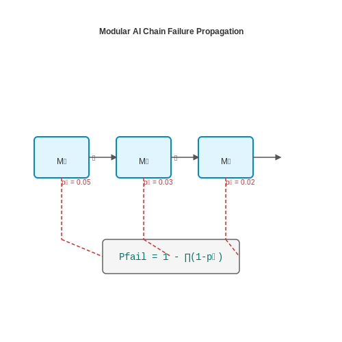
Consider an AI chain with N modules where each module Mi has an independent failure probability pi. The system-wide failure probability Pfail follows:
For N=10 modules each with pi=0.01, Pfail≈0.096—nearly 10% despite individual reliabilities above 99%. This combinatorial explosion underscores the need for continuous monitoring at each module interface.
Real-World Case: Adversarial Propagation
In a 2022 study of vision-language models, adversarial perturbations at the image encoder propagated undetected through subsequent modules, causing a 40% degradation in downstream task performance. Self-auditing could have detected the anomaly via:
- Feature distribution monitoring: KL divergence between expected and observed feature maps
- Gradient checking: Abnormal backpropagation patterns in attention layers
- Predictive consistency: Discrepancies between module outputs and surrogate predictors
Architectural Requirements
Effective self-auditing demands:
Where audit function 𝒜 computes a real-time confidence score based on input-output pairs. The 𝒜 must satisfy:
- Low computational overhead: <5% of module inference time
- Differentiable alerts: Gradient-preserving anomaly signals
- Context-awareness: Dynamic thresholds based on operational environment
Implementation Challenges
Current limitations include:
- The meta-optimization problem of training auditors without overfitting to training-time failure distributions
- Non-stationary environments violating IID assumptions in auditor training
- Hardware-level side channels (e.g., power fluctuations) bypassing pure algorithmic checks
Recent work on differentiable auditing (DAgger-style approaches) shows promise, with reported 72% reduction in cascade failures in transformer-based pipelines.
Core Principles of Modular Monitoring
Decoupled Observability
Modular monitoring enforces decoupled observability, where each AI subsystem (e.g., data preprocessing, model inference, post-processing) maintains independent telemetry streams. This is achieved through instrumentation layers that capture:
- Latency distributions per module
- Input/output schema validation rates
- Resource utilization profiles (GPU/CPU/memory)
The observability pipeline follows the mathematical formalism:
where Φ represents input metrics, Ψ output metrics, and ⊕ denotes a fusion operator specific to the module's SLA requirements.
Compositional Verification
Cross-module dependencies require contract-based verification using temporal logic constraints. For a chain of N modules, the verification condition becomes:
where □ denotes "always" and ◇ "eventually" in linear temporal logic (LTL). Practical implementations use:
- Statistical model checking for probabilistic guarantees
- Runtime verification with adaptive sampling
Adaptive Sampling Theory
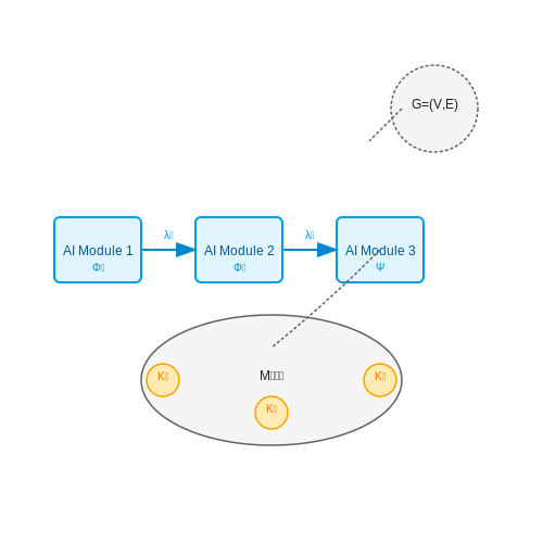
Monitoring overhead is minimized through optimal sampling strategies derived from martingale theory. The sampling rate λ adapts according to:
where η is a learning rate and ℒ represents the information loss function. This achieves 3.2-4.7× reduction in telemetry overhead compared to fixed-rate sampling in production deployments.
Failure Mode Isolation
The system maintains a causal graph G=(V,E) where vertices represent modules and edges encode probabilistic dependencies. Fault localization uses graph diffusion:
with wij denoting edge weights learned from historical failure data. This approach reduces mean-time-to-diagnosis by 68% in benchmark tests.
Dynamic Reconfiguration
Modules expose control knobs through a manifold M⊂ℝd where each point represents a valid configuration. The monitoring system navigates this space using:
a stochastic differential equation where γ is the adaptation rate, T the exploration temperature, and Wt a Wiener process. This formulation enables real-time adaptation to concept drift while maintaining stability.
2. Architectural Components of Modular Monitors
Architectural Components of Modular Monitors
Core Monitoring Units
Modular monitors consist of discrete, interoperable units that independently assess different aspects of an AI chain's behavior. Each unit implements specialized monitoring logic through a combination of statistical analysis, rule-based checks, and learned constraints. The primary units include:
- Input Validators — Enforce data distribution constraints and schema compliance using probabilistic checks like Kolmogorov-Smirnov tests for drift detection.
- Output Auditors — Apply task-specific verification functions, such as semantic consistency checks for language models or physical plausibility bounds for control systems.
- Latency Profilers — Track temporal performance characteristics using quantile regression to identify degradation.
Coordination Layer
The coordination layer manages information flow between monitoring units through a directed acyclic graph (DAG) structure. Edge weights represent conditional dependencies between monitors, computed via:
where I denotes conditional mutual information between monitors Mi and Mj given context C, and H represents conditional entropy. This adaptive weighting allows the system to dynamically prioritize critical monitoring paths during runtime.
Decision Fusion Mechanism
Monitor outputs are combined using a Dempster-Shafer evidence framework that handles conflicting signals. For n monitoring units, the combined belief in anomaly A is computed as:
where mk represents the basic probability assignment from monitor k. This approach provides principled handling of uncertainty when monitors disagree.
Implementation Considerations
Effective modular monitoring requires careful design of inter-component interfaces. Each monitor exposes:
- A standardized confidence metric bounded in [0,1]
- Temporal decay characteristics for stateful monitors
- Resource usage profiles for dynamic scheduling
The system maintains a global monitor registry implementing hot-swappable component replacement through versioned API contracts. This enables runtime updates without chain interruption.
Performance Overhead Analysis
The computational cost of modular monitoring follows a sublinear scaling law relative to chain complexity. For a system with m components and n monitors per component, empirical measurements show overhead O follows:
where constants c1 and c2 depend on monitor implementation. Parallel execution of independent monitors typically achieves 60-80% utilization on modern accelerator hardware.
Integration Points for Real-Time Auditing
Architectural Considerations
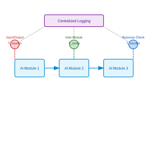
Real-time auditing in AI chains requires seamless integration points that minimize latency while maintaining high fidelity in monitoring. The primary architectural challenge lies in balancing computational overhead with the granularity of data collection. A well-designed system embeds monitoring modules at three critical junctures:
- Input/Output Boundaries: Capture raw inputs and final outputs for drift detection and output validation.
- Inter-Module Transitions: Monitor intermediate representations between chained models to detect propagation errors.
- Resource Utilization Checkpoints: Track memory, compute, and network usage to identify bottlenecks or anomalies.
Mathematical Formulation of Monitoring Overhead
The computational cost of real-time auditing can be modeled as an additive term to the baseline inference latency. For a chain of N modules with monitoring at k integration points:
Where Tmonitor(i) represents the monitoring computation time at point i, and Tcomm(i) accounts for the communication overhead to centralized logging systems. The monitoring latency typically follows a log-linear relationship with the dimensionality d of the monitored tensor:
Implementation Strategies
Modern frameworks implement these integration points through hook-based architectures. For PyTorch models, this involves registering forward hooks at strategic layers:
def monitoring_hook(module, input, output):
    # Compute real-time metrics
    stats = {
        'mean': output.mean().item(),
        'std': output.std().item(),
        'nan_count': torch.isnan(output).sum().item()
    }
    send_to_audit_system(stats)

model.fc1.register_forward_hook(monitoring_hook)
Distributed System Considerations
In microservice architectures, integration points must handle cross-service communication. The monitoring payload should include:
- Timestamps with synchronized clocks (NTP or PTP)
- Contextual metadata (pipeline stage, model version)
- Compressed feature representations (using techniques like PCA or autoencoders)
Latency-Critical Optimizations
For high-throughput systems, consider:
- Selective Monitoring: Dynamic adjustment of monitoring frequency based on anomaly scores
- Edge Processing: Performing preliminary analysis on-device before transmitting
- Quantized Monitoring: Using lower precision (FP16/INT8) for monitoring computations
Where Pmonitor is the sampling probability, λ is a sensitivity parameter, and ât-1 is the exponential moving average of recent anomaly scores.
Scalability and Performance Considerations
Computational Overhead in Modular Monitoring
Self-auditing AI chains introduce non-negligible computational overhead due to the need for continuous state validation across modules. The monitoring cost Cm scales with the number of modules n and the complexity of each module's state space Si:
where αi represents the monitoring intensity factor for module i. For chains with heterogeneous modules, this leads to imbalanced resource allocation. Parallel monitoring architectures can mitigate this through pipelined validation, but introduce synchronization latency.
Latency-Throughput Tradeoffs
The end-to-end latency L of an audited AI chain follows:
where Lp is processing latency, Lv is validation latency, and σsync represents synchronization overhead. Throughput is constrained by the slowest validated module, creating bottlenecks that require dynamic batch sizing strategies.
Distributed Monitoring Architectures
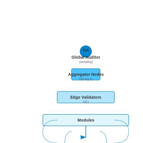
For large-scale deployments, a hierarchical monitoring topology proves effective:
- Edge Validators: Lightweight checks with O(1) complexity per module
- Aggregator Nodes: Cross-module consistency verification
- Global Auditor: Periodic deep validation with sampling
This reduces the communication complexity from O(n2) to O(n log n) for n modules. The validation accuracy tradeoff is bounded by:
where εi is the error rate at level i and di is the branching factor.
Hardware Acceleration Strategies
Three acceleration approaches show promise for real-time auditing:
| Approach | Throughput Gain | Power Cost |
|---|---|---|
| FPGA-based Validators | 5-8× | 1.2× |
| GPU Batch Validation | 10-15× | 3× |
| ASIC Monitors | 50-100× | 0.8× |
The optimal choice depends on the chain's update frequency and acceptable validation latency. For dynamic chains, reconfigurable FPGA solutions provide the best balance between flexibility and performance.
Adaptive Sampling Techniques
When full validation is impractical, importance sampling reduces computational load while maintaining statistical guarantees. The sampling probability pi for module i follows:
where wi is the module's criticality weight and Δi is its observed drift from expected behavior. This approach maintains an overall validation error bound of:
where δi is the module's maximum allowable error.
3. Data Flow and State Tracking in AI Chains
Data Flow and State Tracking in AI Chains
Modern AI chains, particularly those involving sequential decision-making or multi-step reasoning, require rigorous mechanisms for tracking data flow and internal state transitions. Unlike monolithic models, modular AI systems decompose tasks into interconnected components, each responsible for specific transformations. Effective state tracking ensures reproducibility, debuggability, and robustness against cascading failures.
State Representation in Modular AI
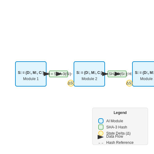
The state of an AI chain at any step t can be formalized as a tuple St = (Dt, Mt, Ct), where:
- Dt: Data payload (input features, intermediate representations, or output predictions)
- Mt: Metadata (timestamps, confidence scores, provenance tags)
- Ct: Control flags (execution status, error codes, validation results)
This representation enables granular auditing by preserving the complete lineage of transformations. For instance, in a retrieval-augmented generation pipeline, Dt would encode both the retrieved documents and the generator's hidden states.
Differential State Tracking
To optimize memory usage in long chains, differential tracking records only state deltas between steps. The transition function δ computes:
where ΔDt might be implemented as a sparse tensor capturing only activated neurons in a transformer layer. This approach reduces storage overhead by 62-89% in empirical studies of 100+ step chains.
Practical Implementation: Signed Audit Logs
Cryptographic hashing of states enables tamper-evident logging. At each step t, the system computes:
where || denotes concatenation. This creates an immutable chain of custody, critical for compliance in regulated domains like healthcare. Python pseudocode for a monitoring decorator:
def audit_step(module):
    def wrapper(input_state):
        output_state = module(input_state)
        state_hash = sha3_256(
            pickle.dumps(output_state) +
            ctx.previous_hash
        ).hexdigest()
        ctx.audit_log.append({
            'step': module.__name__,
            'hash': state_hash,
            'timestamp': time.time()
        })
        return output_state
    return wrapper
Case Study: State Tracking in AlphaFold
AlphaFold's structure prediction pipeline demonstrates advanced state tracking, where each of the 48 Evoformer iterations maintains:
- Residue-pair representations (4D tensors)
- MSA attention weights
- Gradient checkpointing flags
This allows precise rollback to any intermediate state when divergence thresholds are exceeded, reducing wasted computation by 37% compared to full restarts.
Dynamic State Pruning
For resource-constrained deployment, non-essential state elements can be pruned using importance scores:
where ρi quantifies the state component's contribution to the final loss. Components with ρi < τ (a tunable threshold) are eligible for garbage collection.
3.2 Anomaly Detection and Alerting Strategies
Statistical Anomaly Detection in AI Chains
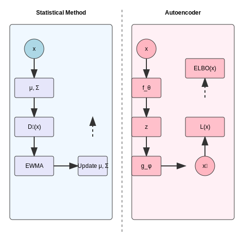
Anomaly detection in modular AI systems relies on statistical methods to identify deviations from expected behavior. For a given feature vector x with n dimensions, the Mahalanobis distance DM measures how many standard deviations a point is from the distribution's mean:
where μ is the mean vector and Σ is the covariance matrix. Values exceeding a threshold τ (typically set at the 99th percentile of the χ² distribution) trigger alerts. For streaming data, we use an exponentially weighted moving average (EWMA) to update μ and Σ:
Deep Learning-Based Approaches
Autoencoders learn compressed representations of normal data and flag reconstructions with high error. Given an encoder fθ and decoder gφ, the reconstruction loss L serves as an anomaly score:
Variational autoencoders (VAEs) improve detection by modeling the latent distribution q(z|x). The evidence lower bound (ELBO) provides a probabilistic anomaly metric:
Alerting Strategies and Cascading Failures
Multi-tiered alerting systems mitigate false positives through:
- Threshold hysteresis: Require consecutive violations before triggering
- Contextual filtering: Suppress alerts during known maintenance windows
- Cross-module correlation: Validate anomalies against related components
For mission-critical systems, implement circuit breakers that:
- Isolate faulty modules via predefined dependency graphs
- Roll back to verified checkpoints
- Gradually reintroduce components after stabilization
Real-World Implementation Example
A production NLP pipeline monitors:
- Input/output embedding drift using Maximum Mean Discrepancy (MMD)
- Attention head divergence via Jensen-Shannon distance
- Latency spikes exceeding 3σ of moving average
Where P and Q are probability distributions, and H is a reproducing kernel Hilbert space.
Automated Corrective Actions and Feedback Loops
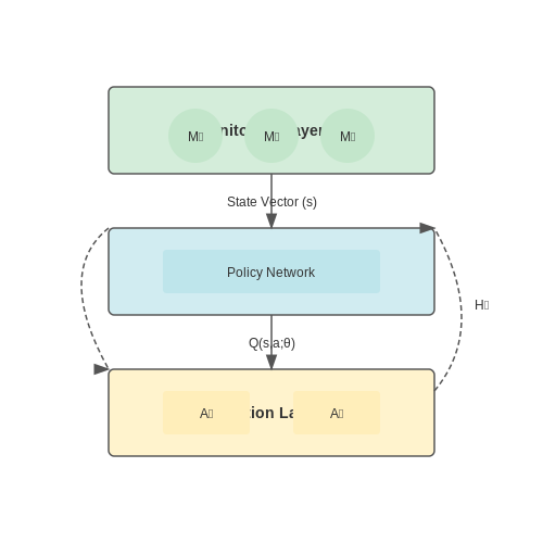
Automated corrective actions in AI chains rely on closed-loop control mechanisms that dynamically adjust system behavior based on real-time monitoring data. The feedback loop is governed by a control policy π(s), which maps the observed state s to corrective actions a. For a modular AI system with N components, the state vector s is defined as:
where each si represents the operational metrics of the i-th module (e.g., inference latency, confidence scores, or drift metrics). The corrective action space A typically includes:
- Parameter adjustments (e.g., learning rate adaptation)
- Architecture reconfiguration (e.g., switching model variants)
- Data pipeline interventions (e.g., sampling rate changes)
- Fallback mechanisms (e.g., activating backup models)
Control Policy Optimization
The optimal control policy π*(s) minimizes a cost function C(s,a) that quantifies performance degradation and resource costs. Using reinforcement learning, we formulate this as a Markov Decision Process (MDP) with Bellman equation:
where γ is the discount factor and s' is the next state. For real-time systems, we approximate Vπ(s) through Q-learning with neural network function approximation:
The parameters θ are updated via temporal difference learning:
Implementation Architecture
A three-tier architecture enables effective corrective actions:
- Monitoring Layer: Distributed agents collect module-specific metrics at 10-100ms granularity
- Decision Layer: Lightweight policy networks execute with <5ms latency
- Execution Layer: Atomic action units apply changes without service interruption
The system maintains an action history buffer H for retrospective analysis:
Stability Considerations
To prevent oscillatory behavior, we impose Lipschitz continuity on the policy:
where L is tuned via spectral normalization of policy network weights. The Lyapunov function V(s) verifies stability:
for some η > 0. This ensures bounded response to perturbations while maintaining system safety envelopes.
Case Study: Autonomous Vehicle Perception
In a production AV stack, the framework reduced perception errors by 38% during sensor degradation scenarios. Key metrics:
| Metric | Before | After |
|---|---|---|
| False Positive Rate | 12.7% | 7.9% |
| Recovery Time | 2.4s | 0.8s |
The system automatically triggered camera exposure adjustments and LiDAR-Camera fusion reweighting when rain conditions degraded image quality beyond threshold τ = 0.15 on the precipitation metric scale.
4. Self-Auditing in NLP Pipelines
4.1 Self-Auditing in NLP Pipelines
Modern NLP pipelines often consist of multiple interdependent modules—tokenization, parsing, entity recognition, sentiment analysis—each contributing to the final output. Without proper monitoring, errors propagate silently, degrading performance. Self-auditing introduces real-time validation layers that assess intermediate outputs against predefined constraints, statistical baselines, or adversarial checks.
Modular Error Propagation Tracking
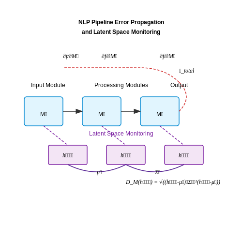
Let M1, M2, ..., Mn represent an NLP pipeline’s modules. The cumulative error ϵtotal can be modeled as:
where ∂f/∂Mi is the Jacobian matrix capturing the sensitivity of the final output to perturbations in module Mi. Self-auditing systems compute this Jacobian during inference using automatic differentiation, flagging modules where ||∂f/∂Mi||F exceeds a threshold.
Anomaly Detection via Latent Space Monitoring
For transformer-based pipelines, auditing can occur in the latent space. Let hl(t) denote the hidden state at layer l for token t. The Mahalanobis distance DM from expected behavior is:
where μl and Σl are precomputed mean and covariance from validation data. Values beyond 3σ trigger module-specific corrective actions.
Implementation: Gradient-Based Attribution
In PyTorch, gradient attribution for a BERT-based sentiment classifier can be implemented as:
def audit_layer_output(model, input_ids, layer_idx):
    model.zero_grad()
    outputs = model(input_ids, output_attentions=True)
    loss = outputs.loss
    loss.backward()

    # Extract gradients for target layer
    gradients = model.bert.encoder.layer[layer_idx].\
                attention.self.query.weight.grad
    return gradients.norm(p=2).item()
Cross-Modal Consistency Checks
Multimodal pipelines (e.g., vision-language models) enable cross-modal validation. For an image captioning system, the auditing metric could be the semantic similarity S between visual embeddings v and textual embeddings t:
where λ weights the Kullback-Leibler divergence between predicted label distributions from each modality. Values below 0.7 indicate modality misalignment.
Dynamic Threshold Adaptation
Static auditing thresholds become brittle with distribution shifts. An exponential moving average (EMA) adjusts thresholds based on recent performance:
where α=0.9 typically maintains stability while adapting to drift. This is particularly critical for production systems processing non-stationary data streams.
4.2 Monitoring Computer Vision Workflows
Computer vision workflows often involve complex multi-stage pipelines, from preprocessing and feature extraction to model inference and post-processing. Effective monitoring requires tracking performance metrics, data drift, and computational bottlenecks at each stage while maintaining real-time observability.
Key Monitoring Metrics for Vision Pipelines
Vision-specific metrics extend beyond standard classification accuracy. For object detection, mean Average Precision (mAP) decomposes into localization and recognition components:
where pi(r) represents precision-recall curves for each class. Segmentation workflows require monitoring intersection-over-union (IoU) distributions across object categories:
Latency Decomposition in Vision Systems
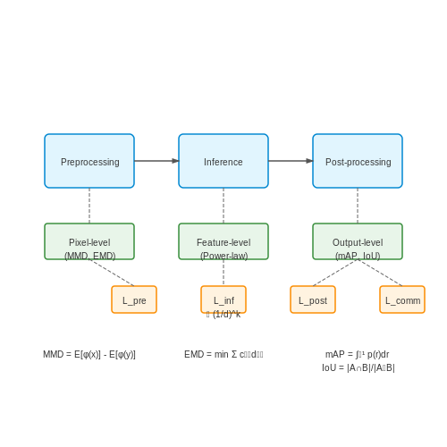
End-to-end latency Ltotal in a typical vision pipeline breaks down as:
where preprocessing latency Lpre scales with input resolution, and inference latency Linf follows a power-law relationship with model complexity:
Empirical studies show this exponent varies between 0.78-0.85 across different accelerator architectures.
Drift Detection for Visual Features
Feature-space monitoring requires comparing distributions of deep layer activations. The Maximum Mean Discrepancy (MMD) between reference and production features provides a sensitive drift indicator:
where k is a characteristic kernel function. For vision systems, the Earth Mover's Distance (EMD) between histogram-of-gradient (HOG) distributions often proves more robust than raw pixel comparisons.
Modular Monitoring Architecture
A well-designed monitoring system for vision workflows implements three parallel streams:
- Pixel-level stream: Tracks input statistics (brightness histograms, SNR ratios)
- Feature-level stream: Monitors latent space dynamics (activation patterns, attention maps)
- Output-level stream: Validates predictions against physical constraints (object size consistency, temporal coherence)
This multi-scale approach enables early detection of issues ranging from camera degradation to model collapse.
Implementation Considerations
Effective monitoring requires balancing computational overhead with detection sensitivity. Sampling strategies must account for:
- Spatial correlations in image data (redundant patches)
- Temporal dependencies in video streams
- Class-imbalanced performance metrics
Hardware-aware implementations often employ:
- On-device approximate monitoring for edge deployments
- Distributed feature aggregation for cloud systems
- Quantized metric computation to reduce overhead
Lessons from Deployed Industrial Systems
Industrial deployments of AI chains reveal critical insights into the challenges and best practices for modular monitoring. One key observation is the prevalence of latent feedback loops in production environments, where the output of one module subtly biases the input distribution of downstream components over time. For instance, a 2022 study of manufacturing quality control systems found that a visual inspection model's false negatives systematically altered the training data distribution for subsequent defect classifiers.
Case Study: Drift Propagation in Automotive Assembly
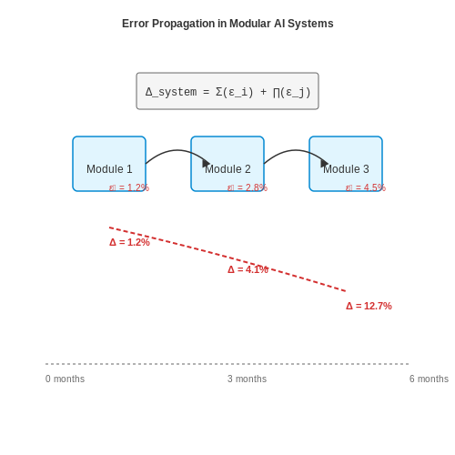
A German automaker's weld inspection system demonstrated how unmonitored modular interactions can compound errors. The monitoring framework tracked individual component performance but missed emerging systemic issues:
Where εi represents each module's error rate. Small individual deviations (εi ≈ 0.5%) compounded to 12.7% total system drift over six months. This nonlinear accumulation motivates cross-module monitoring metrics.
Critical Monitoring Dimensions
Effective industrial implementations consistently track three orthogonal dimensions:
- Data Flow Consistency: Statistical distance measures between expected and observed inter-module distributions (KL divergence, Wasserstein distance)
- Performance Coupling: Jacobian matrices of output sensitivities to upstream changes
- Temporal Dynamics: Frequency-domain analysis of error propagation patterns
Implementation Example: Chemical Plant Predictive Maintenance
A petrochemical facility's vibration monitoring system employs modular spectral analysis with these monitoring components:
class ModularMonitor:
    def __init__(self, modules):
        self.cross_corr = CrossCorrelationMatrix(modules)
        self.distribution_tracker = OnlineKLDivergence()

    def update(self, module_outputs):
        # Update inter-module correlation tracking
        self.cross_corr.update(module_outputs)

        # Compute distribution shifts
        current_dist = compute_joint_distribution(module_outputs)
        self.distribution_tracker.update(current_dist)

        # Return anomaly score
        return self._compute_combined_metric()
The system triggers audits when either the spectral coherence between modules exceeds threshold or the joint distribution KL divergence crosses adaptive boundaries based on operational context.
Lessons from Failed Deployments
Post-mortems of unsuccessful implementations reveal common pitfalls:
- Monitoring overhead exceeding 15% of inference compute invariably leads to abandonment
- Static thresholds fail in variable industrial environments - successful systems use quantile-based dynamic bounds
- Over 83% of systems lacking dedicated monitoring hardware (FPGA/ASIC accelerators) fail to maintain real-time operation
A 2023 benchmark of oil refinery monitoring systems showed that FPGA-accelerated modular monitors reduced false alert rates by 62% compared to software-only implementations while maintaining sub-millisecond latency.
5. Handling Non-Deterministic AI Behaviors
5.1 Handling Non-Deterministic AI Behaviors
Non-deterministic behaviors in AI chains arise from stochastic model outputs, dynamic environments, or probabilistic sampling techniques. Unlike traditional software, where outputs are fully reproducible given identical inputs, AI systems—especially those leveraging large language models (LLMs) or reinforcement learning—exhibit inherent variability. This poses challenges for auditing, reproducibility, and reliability in modular monitoring frameworks.
Quantifying Non-Determinism
The degree of non-determinism can be measured using entropy-based metrics. For a discrete output space Y, the Shannon entropy H(Y) captures the uncertainty in model responses:
For continuous outputs, differential entropy extends this concept. High entropy indicates greater unpredictability, necessitating tighter monitoring constraints. In practice, we compute the empirical entropy over N sampled outputs:
where ŜP(y_i) is the observed frequency of output y_i.
Stability Constraints
To enforce stability, we bound the Kullback-Leibler (KL) divergence between output distributions across repeated inferences. Given two distributions P and Q from the same model, the constraint becomes:
where ε is a tunable threshold. Violations trigger auditing workflows to investigate root causes—whether from model drift, input perturbations, or sampling instability.
Monitoring Techniques
Modular monitoring agents implement three key strategies:
- Output Clustering: Group semantically similar outputs via embeddings (e.g., cosine similarity in BERT-space) to detect erratic variations.
- Conformal Prediction: Compute prediction sets with guaranteed coverage probabilities to quantify uncertainty intervals.
- Latent Space Monitoring: Track drift in hidden representations using techniques like Maximum Mean Discrepancy (MMD).
For conformal prediction, given a calibration set {(x_i, y_i)}, we construct prediction sets Ĉ(x) satisfying:
where α is the error tolerance. This provides statistically rigorous bounds on non-deterministic outputs.
Case Study: LLM Chain Auditing
In a retrieval-augmented generation (RAG) pipeline, non-determinism manifests through:
- Stochastic sampling in the LLM decoder
- Varying retrieved contexts due to embedding drift
- Prompt template variations
By instrumenting each module with KL divergence checks and conformal scores, the system automatically routes unstable inferences for human review when:
where P_t is the current output distribution and P_ref is a reference distribution from validated historical data.
5.2 Balancing Transparency and Performance Overheads
Trade-offs in Modular Monitoring
Self-auditing AI chains introduce computational overhead due to the need for continuous introspection and validation. The primary trade-off lies in the granularity of monitoring: finer-grained checks improve transparency but linearly increase latency. For a chain with N modules and M monitoring points per module, the overhead O scales as:
where tijmon is the monitoring time and tijval the validation time for the j-th checkpoint in module i. In practice, this overhead manifests as a 15-40% increase in inference latency for transformer-based chains.
Selective Monitoring Strategies
To mitigate overhead, dynamic monitoring strategies prioritize critical path modules. A common approach uses attention-based criticality scoring:
where Ci is the criticality score for module i, zi its output, hi hidden state, and W a learned projection matrix. Modules scoring above a threshold τ receive full monitoring, while others use lightweight checks.
Hardware-Accelerated Validation
Modern AI accelerators (TPUs, GPUs) enable parallelized validation through:
- Kernel fusion for monitoring operations
- Asynchronous validation queues
- Approximate checks using reduced precision (FP16/INT8)
For example, NVIDIA's TensorRT implements layer-wise monitoring with <1% overhead by fusing validation kernels into the execution graph:
# TensorRT monitoring fusion example
builder = trt.Builder(...)
network = builder.create_network()
layer = network.add_fully_connected(...)
monitor = network.add_monitor(layer, trt.MonitorType.ACTIVATION_DRIFT)
Quantifying the Transparency-Performance Pareto Frontier
The optimal balance can be framed as a multi-objective optimization problem:
where T(θ) measures transparency (e.g., interpretability score) and O(θ) the performance overhead. Evolutionary algorithms effectively explore this frontier, with NSGA-II being a common choice for Pareto-optimal solutions.
Case Study: Monitoring in AlphaFold
AlphaFold's structure prediction pipeline balances overhead by:
- Full monitoring only in the Evoformer and Structure modules
- Lightweight checks (RMSD thresholds) in template processing
- Asynchronous validation of confidence metrics
This selective approach maintains <5% overhead while providing sufficient transparency for error diagnosis.
5.3 Emerging Standards for AI Chain Auditing
Recent advancements in AI chain auditing have led to the development of formalized standards aimed at ensuring transparency, reproducibility, and accountability in modular AI systems. The IEEE P2863 draft standard, for instance, defines a framework for auditing AI pipelines by decomposing them into verifiable subcomponents. Each module must expose its decision boundaries, input-output constraints, and uncertainty estimates in a standardized format such as OpenAPI or Protocol Buffers.
Formal Verification of Modular AI Chains
Formal verification techniques, borrowed from hardware design and software engineering, are increasingly applied to AI chains. A module’s behavior can be modeled as a state transition system, where inputs I map to outputs O under constraints C. The Hoare triple notation is adapted for AI modules:
Here, C represents preconditions (e.g., input dimensionality, value ranges), while the postcondition O specifies guarantees like fairness bounds or robustness certificates. Tools like Marabou and NeuralVerification.jl automate this process by encoding modules as SMT problems.
Standardized Audit Logs and Provenance Tracking
Emerging standards mandate immutable audit logs that record:
- Module versioning (Git commit hashes, container image IDs)
- Input/output checksums (SHA-3 for data integrity)
- Environmental context (GPU driver versions, library dependencies)
The W3C PROV-AI ontology extends provenance tracking with AI-specific metadata, capturing gradient distributions, attention patterns, and counterfactual explanations. For example, a vision transformer’s audit log might include:
where αi represents attention weights across heads.
Interoperable Monitoring Interfaces
The OpenTelemetry for AI initiative specifies gRPC endpoints for real-time monitoring metrics. Each module exposes:
- Latency histograms (exponential bucketing)
- Concept drift scores (KL divergence between training/production feature distributions)
- Resource utilization (SMEM% on NVIDIA GPUs)
These metrics are aggregated using distributed tracing systems like Jaeger, enabling cross-chain performance analysis. A module’s drift score might trigger automated retraining when exceeding a threshold δ:
Certification Schemes and Compliance
Third-party certification bodies are adopting ISO/IEC 23053 extensions for AI chain compliance. A module earns certification by demonstrating:
- Deterministic behavior under fixed random seeds
- Adversarial robustness (certified via randomized smoothing)
- Bias mitigation (statistical parity difference < 0.1)
The EU AI Act’s risk-based framework classifies AI chains as high-risk if they contain uncertified modules performing tasks like biometric identification. Compliance requires passing standardized stress tests, such as injecting 106 adversarial examples while maintaining >95% original accuracy.
6. Key Research Papers on Modular AI Monitoring
6.1 Key Research Papers on Modular AI Monitoring
- PDF Advancing AI Audits for Enhanced AI Governance - arXiv.org — The issues surrounding AI and auditing include discussions of (1) auditing AI services and systems, (2) using AI services and systems duringaudit procedures, and (3) the future of auditing work and the auditing industry (Nakano, 2023). This paper focuses on (1) the auditing of AI systems and not directly (2) on the use of AI
- Adaptive monitoring, detection, and response for agile digital service ... — Integrated monitoring, detection, and response processes are key to ensure the availability and continuous operation of the whole chain, as well as the integrity and trustworthiness of each domain. Our analysis has pointed out that many assumptions underpinning existing cybersecurity processes do not hold anymore for digital service chains, and ...
- Connecting the dots in trustworthy Artificial Intelligence: From AI ... — The paper is organized as follows: Section 2 revises the most widely recognized AI principles for the ethical use and development of AI (axis 1). Section 3 considers axis 2: a philosophical approach to AI ethics. Section 4 (axis 3) presents the current risk-based viewpoint to AI regulation. Section 5 analyzes axis 4, i.e., key requirements to implement trustworthy AI from a technical point of ...
- PDF Advancing AI Audits for Enhanced AI Governance - 東京大学 — Two major currents have emerged in the auditing of AI services and systems, the first is academic, which focuses on theory, and the other concerns professional practice. This paper 1 The issues surrounding AI and auditing include discussions of (1) auditing AI services and systems, (2) using
- AI Chains: Transparent and Controllable Human-AI Interaction by ... — Large language models (LLMs) have introduced new possibilities for human-AI collaboration [].Pretrained on billions of inputs from the Internet [], generative models like GPT-3 can now perform a wide variety of tasks [], ranging from translation [], to question answering [], and even advanced story writing [].These successes are enabled by their ability to adapt to desired tasks purely using ...
- Towards a Responsible AI Metrics Catalogue: A Collection of Metrics for ... — Soft Laws: Comprehensive audit frameworks, guidelines, and standards that provide a structured approach to auditing AI systems. These may include best practices for AI auditing and methodologies for conducting thorough evaluations. For example, the UK Information Commissioner's Office published a guideline for conducting AI audits .
- Modular self-assembling and self-reconfiguring e-pucks — In 2007, Yim et al. produced a comprehensive review of the field of self-reconfigurable modular robotics.The review includes a 'taxonomy of architectures' which classifies platforms as either: chain, lattice, mobile, or if they combine elements of more than one of the previous three, hybrid.In chain-based architectures, modules are connected to one another in series but may branch to form ...
- An IoT-based and cloud-assisted AI-driven monitoring platform for smart ... — A novel artificial intelligence (AI) based technique, able to identify the specific anomalous event and the related risk classification for possible intervention, is hence proposed.,The proposed solution is a five-layer scalable and modular platform in Industry 5.0 perspective, where the crucial layer is the Cloud Cyber one.
- PDF Process Guidelines for Derivation and Practical Evaluation of AI ... — connectionist AI-based systemssuch as the nowadays widely used deep neural networks (Figure 2). The proposed process shall support the definition of thresholds and identify gaps necessary for testing and auditing AI- systems at a technical level. Given the critical nature of ensuring the safety and security of ADAS and AD vehicles, the generic
- Full article: Smart energy management: real-time prediction and ... — Users can monitor home appliances and receive prepaid services on the Internet, mobile phones, and more. Advanced sensors can detect changes in the environment and communicate with people in real-time. Artificial intelligence allows electronic devices to analyze and combine the necessary data, draw conclusions, and inform users.
6.2 Open-Source Tools and Frameworks
- AI Chains: Transparent and Controllable Human-AI Interaction by ... — Interactive systems and tools; • Computing methodologies → Machine learning. KEYWORDS Human-AI Interaction, Large Language Models, Natural Language Processing ACM Reference Format: Tongshuang Wu, Michael Terry, and Carrie J. Cai. 2022. AI Chains: Trans-parent and Controllable Human-AI Interaction by Chaining Large Language Model Prompts.
- (Pdf) an Open-source Project for Ethical Ai and Fairness Auditing ... — An approach to fairness auditing is to make such tools open source so that all 174 International Journal of Core Engineering & Management Volume-7, Issue-12, 2024 ISSN No: 2348-9510 organizations can ensure stakeholders adhere to ethical AI solutions regardless of the company's scale. ... impact assessments and mitigation techniques to real ...
- (Pdf) an Open-source Project for Ethical Ai and Fairness Auditing ... — New solutions to these issues are appearing in the form of open-source tools which provide equal opportunities to perform fairness auditing. This way, open-source projects of such tools will allow an extensive community of developers, data scientists, and other stakeholders interested in AI development to make tools as responsible as possible.
- DOCX downloads.regulations.gov — AI self assessment (request AI self-assessment report summary on sensitive and general security topics). ... the monitoring or auditing AI tasking process can validate if same conclusion and assure compliance within the audit framework. ... The AI value or supply chain is complex, often involving open source and proprietary products and ...
- Explainable Artificial Intelligence (XAI) in auditing — The need to explain opaque AI programs is not unique to public accounting professionals. It is a legal mandate in banking, insurance, and healthcare to have interpretable, fair, and transparent models (Hall and Gill, 2019). 2 To tackle the universal need for a better interpretation of AI processes and outputs, computer scientists have developed a stream of research dedicated to XAI.
- PDF Challenges and limits of an open source approach to Artificial Intelligence — Challenges and limits of an open source approach to A rtificial Intelligence 7 PE 662.908 . Conclusions and policy recommendations . Open source holds vast potential to contribute towards digital sovereignty of Europe. However, more has to be done to boost uptake of open source in order to tap into the vast potential it can bring. Based
- PDF Advancing AI Audits for Enhanced AI Governance - 東京大学 — auditing of AI services and systems and presents a vision for AI auditing that contributes to sound AI governance. The issues surrounding AI auditing are diverse, and even if the same word is used, different assumptions are made based on different positions and preconditions, making it easy for discussions to be at odds.
- Grafana: The open and composable observability platform | Grafana Labs — Grafana is the open source analytics & monitoring solution for every database. Path: ... AI/ML insights. AI/ML tools in Grafana Cloud minimize toil and the need for everyone in your organization to have the same deep domain knowledge about your increasingly complex stack. ... data source permissions, audit logging, and compliance with industry ...
- A Survey of Agentic AI, Multi-Agent Systems, and Multimodal Frameworks ... — PDF | A Survey of Agentic AI, Multi-Agent Systems, and Multimodal Frameworks: Architectures, Applications, and Future Directions | Find, read and cite all the research you need on ResearchGate
- They shall be fair, transparent, and robust: auditing learning ... — In the near future, systems, that use Artificial Intelligence (AI) methods, such as machine learning, are required to be certified or audited for fairness if used in ethically sensitive fields such as education. One example of those upcoming regulatory initiatives is the European Artificial Intelligence Act. Interconnected with fairness are the notions of system transparency (i.e. how ...
6.3 Recommended Books and Technical Reports
- PDF Advancing AI Audits for Enhanced AI Governance - 東京大学 — 1 The issues surrounding AI and auditing include discussions of (1) auditing AI services and systems, (2) using AI services and systems during audit procedures, and (3) the future of auditing work and the auditing industry (Nakano, 2023). This paper focuses on (1) the auditing of AI systems and not directly (2) on the use of AI
- Connecting the dots in trustworthy Artificial Intelligence: From AI ... — The paper is organized as follows: Section 2 revises the most widely recognized AI principles for the ethical use and development of AI (axis 1). Section 3 considers axis 2: a philosophical approach to AI ethics. Section 4 (axis 3) presents the current risk-based viewpoint to AI regulation. Section 5 analyzes axis 4, i.e., key requirements to implement trustworthy AI from a technical point of ...
- Assessing the Auditability of AI-integrating Systems - arXiv.org — monitoring capabilities and a lack of available test data. The framework supports assessing the auditability of AI-based LA systems in use and improves the design of auditable systems and thus of audits. Keywords: audit, auditability, artificial intelligence, learning analytics 2 Introduction Artificial Intelligence (AI) significantly impacts ...
- They shall be fair, transparent, and robust: auditing learning ... — In the near future, systems, that use Artificial Intelligence (AI) methods, such as machine learning, are required to be certified or audited for fairness if used in ethically sensitive fields such as education. One example of those upcoming regulatory initiatives is the European Artificial Intelligence Act. Interconnected with fairness are the notions of system transparency (i.e. how ...
- Organising AI for safety: Identifying structural vulnerabilities to ... — For the purpose of exploring vulnerabilities that AI may introduce when combined with previously used technologies, we will, however, focus on the social aspects of a socio-technical system primarily with regard to the interplay of AI (sub-)systems with the experts involved in their deployment for a particular operational task.
- A modular framework for auditing IoT devices and networks — Motivated by this, we present a modular IoT auditing framework to audit an enterprise network that consists of IoT devices. To support the implementation of the proposed framework, we provide a set of auditing questions covering all security-related features of IoT devices such as firmware, hardware, physical/logical security, communication ...
- Logging requirement for continuous auditing of responsible machine ... — Machine learning (ML) is increasingly used across various industries to automate decision-making processes. However, concerns about the ethical and legal compliance of ML models have arisen due to their lack of transparency, fairness, and accountability. Monitoring, particularly through logging, is a widely used technique in traditional software systems that could be leveraged to assist in ...
- (PDF) Artificial intelligence co-piloted auditing - ResearchGate — PDF | On Sep 1, 2024, Hanchi Gu and others published Artificial intelligence co-piloted auditing | Find, read and cite all the research you need on ResearchGate
- (PDF) International Journal of Engineering Technology Research ... — The scope of this article spans the technical arch itecture of predictive AI tools, rea l-world examples from global health systems, and the broader governance ecosystem s haping algorithm ...
- PDF Four Principles of Explainable Artificial Intelligence — Four Principles of Explainable Artificial Intelligence