AI-Driven Cleaning Robot Route Planning
1. Core Components of Cleaning Robots
Core Components of Cleaning Robots
Sensing and Perception Systems
Modern cleaning robots integrate multiple sensor modalities for environment mapping and obstacle avoidance. Lidar sensors provide high-resolution 2D or 3D point clouds with typical angular resolution of 0.1°-0.5° and range accuracy of ±2cm. Time-of-flight (ToF) cameras offer depth perception at 30-60 fps with VGA resolution, while structured light systems achieve sub-millimeter precision at shorter ranges. Ultrasonic sensors complement these with robust object detection in transparent or reflective surfaces where optical sensors fail.
Simultaneous Localization and Mapping (SLAM) algorithms fuse this sensor data using probabilistic approaches. The robot's pose (x, y, θ) and environment map m are jointly estimated through:
where z represents sensor measurements and u denotes odometry inputs. Particle filters or graph-based optimization techniques solve this estimation problem in real-time.
Navigation and Control
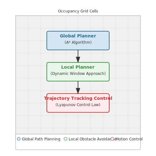
The navigation stack implements a hierarchical architecture. Global planners use A* or Dijkstra's algorithm on occupancy grids to compute optimal paths, while local planners employ dynamic window approaches for reactive obstacle avoidance. The control law for trajectory tracking can be derived from Lyapunov stability theory:
where e represents the tracking error and K terms are gain matrices tuned through pole placement. Advanced systems incorporate model predictive control (MPC) with 5-20ms time horizons to handle nonholonomic constraints.
Power and Actuation
Brushless DC motors with planetary gearheads (typically 50:1 to 100:1 reduction ratios) provide wheel actuation, drawing 2-5A during normal operation. Lithium-ion battery packs (14.4V-25.2V, 2000-5000mAh) power the system with runtime optimization through:
where η accounts for voltage conversion losses (typically 85-92%). Power management ICs implement dynamic voltage scaling to extend battery life during low-load conditions.
Computational Hardware
Embedded processors balance real-time constraints with power efficiency. Modern cleaning robots utilize heterogeneous architectures combining:
- ARM Cortex-M7/M4 cores (200-400MHz) for motor control
- ARM Cortex-A53/A72 (1-2GHz) for SLAM processing
- Neural accelerators (1-4 TOPS) for object classification
Memory hierarchies typically include 512KB-2MB SRAM for real-time tasks and 1-4GB LPDDR4 for mapping algorithms. ROS 2 middleware facilitates inter-process communication with deterministic latencies below 10ms.
Cleaning Mechanisms
Vacuum systems employ centrifugal fans generating 15-25kPa suction, with airflow modeled by:
where d is nozzle diameter and ρ is air density. Brush motors operate at 3000-8000 RPM with current monitoring for hair/tangle detection. Wet cleaning systems use peristaltic pumps with flow rates of 10-30ml/min and closed-loop pressure control.
Role of AI in Autonomous Navigation
Foundations of AI-Driven Navigation
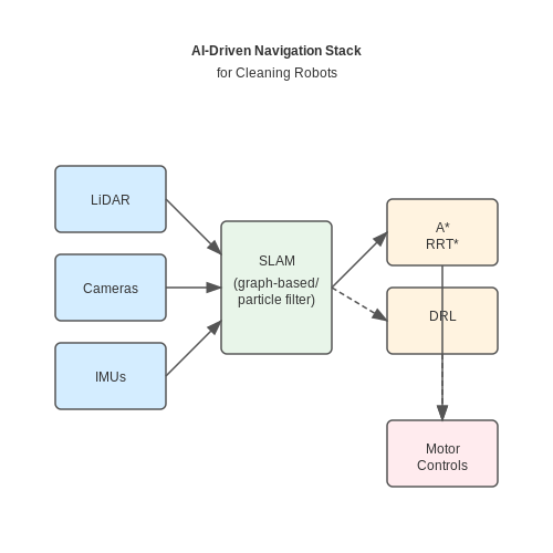
Autonomous navigation in cleaning robots relies on a combination of perception, localization, mapping, and path planning. AI algorithms process sensor data (e.g., LiDAR, cameras, IMUs) to construct a real-time representation of the environment. Simultaneous Localization and Mapping (SLAM) is a cornerstone technique, enabling the robot to build a map while tracking its position within it. Modern implementations often use graph-based SLAM or particle filters (e.g., FastSLAM) to handle dynamic environments.
Here, xt represents the robot's state at time t, z1:t are observations, and u1:t are control inputs. The recursive Bayesian update forms the basis for probabilistic localization.
Path Planning and Optimization
Once the environment is mapped, AI-driven path planning algorithms determine the most efficient cleaning route. Common approaches include:
- A* Search – Heuristic-based graph traversal optimizing for shortest path.
- Dijkstra's Algorithm – Guarantees optimality in static environments.
- RRT* (Rapidly-exploring Random Trees) – Sampling-based method for high-dimensional spaces.
- Deep Reinforcement Learning (DRL) – Neural networks learn optimal policies through trial and error.
For coverage path planning (CPP), a variant of the Traveling Salesman Problem (TSP) is often solved:
where π is a permutation of waypoints and d is the distance metric.
Adaptive Learning in Dynamic Environments
AI enables real-time adaptation to environmental changes. For instance, convolutional neural networks (CNNs) classify obstacles, while recurrent neural networks (RNNs) predict movement patterns of dynamic objects. Reinforcement learning frameworks like Proximal Policy Optimization (PPO) refine navigation policies through continuous interaction:
where rt(θ) is the probability ratio between new and old policies, and Ât is the advantage estimate.
Case Study: Neural Motion Planning
Recent research integrates Graph Neural Networks (GNNs) with traditional planners. For example, a GNN processes the environment's topological graph, predicting feasible trajectories:
where hv(l) is the node embedding at layer l, W(l) is a learnable weight matrix, and ϕ(l) aggregates neighbor information.
1.3 Sensor Integration for Environment Perception
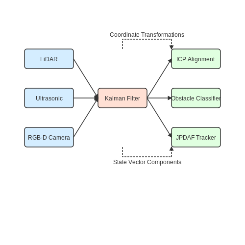
Modern cleaning robots rely on multi-sensor fusion to construct accurate environment maps and optimize path planning. The primary sensors include LiDAR, ultrasonic rangefinders, inertial measurement units (IMUs), and RGB-D cameras, each contributing distinct perceptual capabilities. Sensor fusion algorithms must account for varying update rates, measurement uncertainties, and coordinate frame transformations to generate a consistent environmental representation.
LiDAR Point Cloud Processing
2D LiDAR sensors, such as the RPLIDAR A1, generate polar coordinate measurements with angular resolution down to 0.45°. The raw scan data requires preprocessing:
where ri represents the corrected distance measurement at angle θi, with Gaussian noise variance σnoise2 and systematic error δ. Iterative Closest Point (ICP) algorithms align successive scans by minimizing:
where T is the rigid transformation matrix between point sets pk and qk.
Time-Synchronized Sensor Fusion
Kalman filtering integrates asynchronous sensor data by modeling system dynamics:
where Fk is the state transition matrix and Hk the observation model. For cleaning robots, the state vector typically includes:
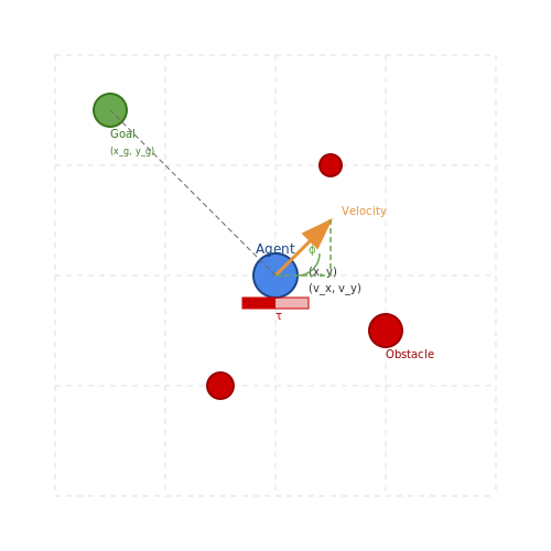
- Position (x, y) with ±2 cm accuracy
- Orientation θ with ±0.5° precision
- Velocity components (vx, vy)
Obstacle Classification
Multi-modal sensor data enables material discrimination through feature extraction:
| Sensor | Feature | Discrimination Threshold |
|---|---|---|
| Ultrasonic | Echo decay rate | τ > 1.2 ms for soft materials |
| RGB-D | Surface texture entropy | H > 5.8 bits for carpets |
| LiDAR | Reflectivity | R < 0.3 for glass surfaces |
Support Vector Machines (SVMs) with radial basis function kernels achieve >92% classification accuracy when trained on these multi-sensor features.
Dynamic Object Tracking
Moving objects are tracked using joint probabilistic data association filters (JPDAF), which compute association probabilities βjt between measurements zj and tracks t:
where λFA is the false alarm density and St the innovation covariance. This enables reliable tracking of pets or moving obstacles at velocities up to 1.5 m/s.
2. Graph-Based Pathfinding Methods
2.1 Graph-Based Pathfinding Methods
Graph-based pathfinding is a fundamental approach in AI-driven cleaning robot navigation, where the environment is represented as a weighted graph G = (V, E), with vertices V representing locations and edges E representing traversable paths between them. The edge weights typically encode traversal costs, which may include distance, energy consumption, or time.
Dijkstra's Algorithm
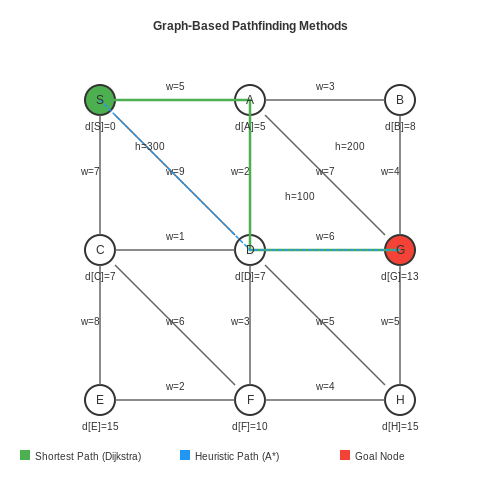
Dijkstra's algorithm computes the shortest path from a single source node to all other nodes in a graph with non-negative edge weights. The algorithm maintains a priority queue of nodes, ordered by their current shortest known distance from the source. At each iteration, the node with the smallest distance is processed, and its neighbors' distances are updated if a shorter path is found.
where d[v] is the distance to node v, u is the current node, and w(u, v) is the edge weight between u and v. The time complexity is O(|E| + |V| log |V|) when implemented with a Fibonacci heap.
A* Search
A* extends Dijkstra's algorithm by incorporating a heuristic function h(v) that estimates the cost from node v to the goal. The priority queue is ordered by f(v) = g(v) + h(v), where g(v) is the known cost from the start to v. If h(v) is admissible (never overestimates the true cost), A* guarantees optimality.
Common heuristics for grid-based environments include Euclidean distance and Manhattan distance. The efficiency of A* depends heavily on the quality of the heuristic.
Probabilistic Roadmaps (PRM)
In high-dimensional or continuous spaces, PRM constructs a graph by randomly sampling configurations and connecting them if a collision-free path exists. The resulting graph can then be searched using Dijkstra's or A*. PRM is particularly useful for robots with complex kinematics or dynamic obstacles.
Multi-Agent Pathfinding (MAPF)
For cleaning robots operating in teams, MAPF algorithms such as Conflict-Based Search (CBS) or Priority-Based Planning ensure collision-free paths. CBS resolves conflicts by splitting the problem into subproblems with constraints, while priority-based methods assign fixed priorities to agents.
where πi is the path of agent i and ci is its cost function.
Dynamic Replanning with D* Lite
When the environment changes (e.g., new obstacles appear), D* Lite efficiently repairs the previous solution by incrementally updating affected parts of the graph. It uses a backward search from the goal and leverages heuristic values to minimize recomputation.
where rhs(s) is the one-step lookahead value and h is the heuristic.
2.2 Heuristic Approaches for Efficient Coverage
Heuristic methods provide computationally tractable solutions to the NP-hard problem of optimal coverage path planning (CPP) for cleaning robots. Unlike exact algorithms, which guarantee optimality at the expense of scalability, heuristics trade optimality for real-time feasibility in large or dynamic environments.
Boustrophedon Decomposition
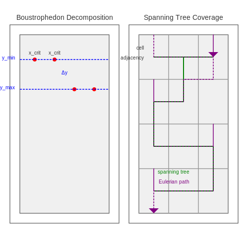
The boustrophedon approach decomposes the workspace into non-overlapping subregions where simple back-and-forth motions achieve complete coverage. The decomposition occurs at critical points where the sweep line's connectivity changes:
where xcrit denotes critical x-coordinates where vertical connectivity changes, and ymin, ymax define vertical bounds. The coverage path P for each region Ri follows:
with Δy representing the robot's cleaning width. This method guarantees complete coverage but may produce inefficient turns at region boundaries.
Spanning Tree Coverage (STC)
STC converts the coverage problem into finding a spanning tree of the environment's grid decomposition. The algorithm proceeds in three phases:
- Grid Formation: Discretize workspace into cells sized by robot footprint
- Dual Graph Construction: Create graph G = (V,E) where vertices represent cells and edges connect adjacent cells
- Tree Generation: Compute minimal spanning tree using Prim's or Kruskal's algorithm
The coverage path follows the tree's Eulerian cycle, with path length bounded by:
Neural Heuristic Approaches
Recent advances employ deep reinforcement learning (DRL) to learn coverage policies. The Markov Decision Process (MDP) formulation includes:
- State space: S = {occupancy grid, robot pose, coverage map}
- Action space: A = {move_forward, turn_left, turn_right}
- Reward function: rt = α⋅Δcovered - β⋅energy_consumed - γ⋅revisits
The Q-function update follows the Bellman equation:
Practical implementations often use Double DQN or PPO to stabilize training. Field tests show neural methods adapt better to irregular environments but require extensive training data.
Multi-Objective Optimization
Advanced systems optimize coverage simultaneously with:
where T is time, E is energy, and M is missed area. Pareto-optimal solutions are found using:
- Genetic algorithms: NSGA-II variants with path encoding chromosomes
- Ant colony optimization: Pheromone matrices biased by coverage objectives
- Monte Carlo tree search: Adaptive sampling of promising path segments
These methods typically achieve 15-30% better multi-objective performance than single-criterion heuristics in complex environments.
2.3 Dynamic Replanning for Obstacle Avoidance
Real-world environments are dynamic, requiring cleaning robots to continuously adapt their paths in response to unforeseen obstacles. Traditional static path planning algorithms like A* or Dijkstra’s become insufficient when the workspace changes during execution. Dynamic replanning addresses this by integrating real-time sensor data into the navigation stack, enabling the robot to modify its trajectory while minimizing disruption to the cleaning task.
Reactive vs. Predictive Obstacle Avoidance
Two primary paradigms exist for dynamic obstacle handling:
- Reactive methods like Dynamic Window Approach (DWA) or Potential Fields provide instantaneous collision avoidance but may lead to suboptimal paths or oscillations.
- Predictive methods leverage probabilistic models (e.g., Kalman Filters) to anticipate obstacle trajectories, enabling smoother avoidance maneuvers.
The optimal solution often combines both approaches. For instance, a cleaning robot might use:
where weights α, β, γ balance path efficiency (e.g., coverage completeness), safety margins, and battery consumption during replanning.
Incremental Graph Updates for Efficient Replanning
Instead of recomputing the entire path from scratch, efficient algorithms like D* Lite maintain and incrementally update a graph representation of the environment. The key steps involve:
- Detecting changed edge costs via LIDAR/vision sensors
- Propagating cost changes locally using heuristics
- Recomputing only affected portions of the path
The time complexity reduces from O(n²) to O(k log n) for k affected nodes, critical for real-time operation on embedded hardware.
Velocity Obstacle Paradigm for Moving Objects
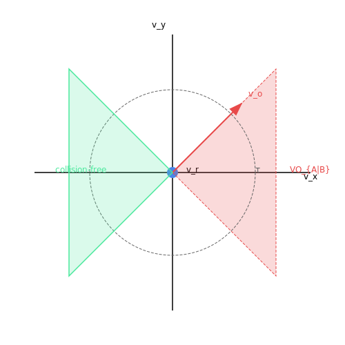
When avoiding moving obstacles (e.g., pets or humans), the Velocity Obstacle (VO) method calculates collision cones in velocity space:
where D is the disc centered at relative position pB - pA with combined radii. The robot selects the nearest collision-free velocity outside these cones while maintaining cleaning coverage objectives.
Implementation Considerations
Practical implementations must address:
- Sensor latency compensation: Kalman Filters predict obstacle positions at planning time
- Partial observability: Bayesian occupancy grids handle uncertain measurements
- Kinematic constraints: Differential drive limitations affect achievable velocities
Modern systems like ROS Navigation Stack implement these concepts through layered costmaps and plugin-based planners, allowing customization for specific cleaning robot configurations.
3. Energy Consumption Minimization
3.1 Energy Consumption Minimization
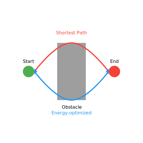
Energy efficiency in AI-driven cleaning robots is critical for extending operational duration and reducing recharge cycles. The problem can be formulated as an optimization task where the robot's path planning algorithm minimizes total energy expenditure while ensuring complete coverage of the cleaning area. The primary energy sinks include locomotion, computation, and active sensing.
Energy Model Formulation
The total energy consumption Etotal of a cleaning robot during operation is the sum of three components:
Where Emotion depends on the distance traveled and surface friction characteristics, Ecompute scales with the complexity of the path planning algorithm, and Esensor is proportional to the active sensing duration.
Motion Energy Optimization
The motion energy component can be modeled using a wheeled robot dynamics framework. For a robot with mass m moving at velocity v on a surface with friction coefficient μ, the instantaneous power consumption is:
Where g is gravitational acceleration, ρ is air density, Cd is the drag coefficient, and A is frontal area. The optimal velocity profile that minimizes energy consumption while maintaining cleaning effectiveness can be derived using calculus of variations:
Computational Energy Trade-offs
Path planning algorithms exhibit different computational complexities and energy profiles. For a grid-based A* search with n nodes, the energy consumption scales as:
Where k1 and k2 are hardware-dependent constants. More sophisticated algorithms like RRT* or neural planners may offer path length improvements but at higher computational cost. The energy-optimal algorithm choice depends on the environment complexity and hardware capabilities.
Sensor Activation Scheduling
Modern cleaning robots employ various sensors (LIDAR, cameras, bump sensors) with different power requirements. An optimal sensing strategy alternates between high-power sensors for localization and low-power sensors for obstacle avoidance. The sensor activation problem can be formulated as a Markov Decision Process where the policy π minimizes:
Where γ is a discount factor and Psensor is the power consumption of action at in state st.
Practical Implementation Considerations
Real-world implementations must account for battery discharge characteristics and regenerative braking effects. Lithium-ion batteries exhibit non-linear discharge curves where the effective capacity decreases with higher current draw. The complete energy optimization problem becomes:
Where ηbattery is the current-dependent battery efficiency. Modern implementations often solve this using model predictive control with a receding horizon approach, updating the optimization every 100-500ms based on current state estimates.
3.2 Time-Optimal Path Planning
Time-optimal path planning in AI-driven cleaning robots involves minimizing traversal time while ensuring complete coverage of the target area. This problem is fundamentally a variant of the Traveling Salesman Problem (TSP) with dynamic constraints, where the robot must navigate obstacles while optimizing acceleration, velocity, and turning delays.
Mathematical Formulation
The time-optimal path can be modeled using a cost function J that integrates kinematic constraints:
where v(t) is velocity, κ(t) is path curvature, and λ penalizes sharp turns. The Hamiltonian H for this system is derived via Pontryagin's minimum principle:
where p is the costate vector, f(x,u) describes system dynamics, and L(x,u) is the Lagrangian. The optimal control input u* satisfies:
Practical Implementation
Modern cleaning robots use hybrid approaches combining:
- Dijkstra's algorithm for global waypoint sequencing
- Model Predictive Control (MPC) for local trajectory optimization
- Bézier curves for smooth motion planning
A typical MPC formulation for a differential-drive robot discretizes the state-space model:
where (x,y) are positional coordinates and θ is orientation. The optimization minimizes:
Case Study: Dynamic Obstacle Avoidance
In cluttered environments, the system must recompute paths in real-time. A hierarchical approach:
- Global planner generates waypoints using A* on a coarse grid
- Local planner refines trajectories using elastic bands method
- Control layer executes time-optimal velocity profiles
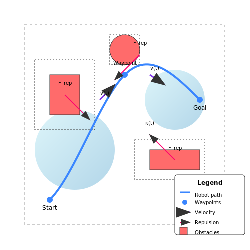
The elastic bands method represents the path as a series of connected springs, where obstacle repulsion forces modify the equilibrium positions:
where η is a scaling factor and d is distance to obstacles.
Computational Considerations
Real-time performance requires:
- Fixed-time termination of optimization solvers
- Efficient collision checking via axis-aligned bounding boxes (AABBs)
- Hardware acceleration of matrix operations
The following SVG illustrates a time-optimized cleaning path with velocity heatmap:
3.3 Multi-Robot Coordination Strategies
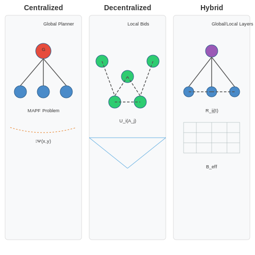
Multi-robot coordination in cleaning applications requires solving complex spatial and temporal allocation problems while minimizing interference and maximizing coverage efficiency. The primary approaches can be categorized into centralized, decentralized, and hybrid architectures, each with distinct trade-offs in scalability, robustness, and computational complexity.
Centralized Coordination
Centralized systems employ a global planner that computes optimal paths for all robots simultaneously. This is typically formulated as a multi-agent path finding (MAPF) problem, where the objective is to minimize the makespan (total cleaning time) while avoiding collisions. The MAPF problem can be expressed as:
where Ti represents the completion time for robot i, and posi(t) denotes its position at time t. Optimal solutions using algorithms like Conflict-Based Search (CBS) achieve completeness but scale exponentially with the number of robots.
Decentralized Approaches
Decentralized coordination relies on local communication and decision-making. Market-based auction mechanisms are particularly effective, where robots bid for regions using a utility function:
Here, Aj represents a cleaning region, ri is the robot's position, and Pk,j is the estimated probability of robot k claiming Aj. This approach enables real-time adaptation but may suffer from local optima.
Hybrid Coordination
Hybrid systems combine global oversight with local autonomy. A common implementation uses a hierarchical architecture:
- Global layer: Partitions the environment into sectors using generalized Voronoi diagrams
- Local layer: Implements modified boustrophedon coverage patterns within each sector
The sector boundary adjustment follows the gradient of the cleaning priority map Ψ(x,y):
where D is dirt density, C is congestion, and α, β are weighting factors.
Dynamic Role Assignment
In heterogeneous robot teams, dynamic role switching optimizes resource utilization. The role assignment matrix R evolves according to:
where Ei represents the efficiency metric for robot i performing role j, and θ is a switching threshold. This formulation enables automatic reconfiguration when environmental conditions change.
Communication Topologies
The choice of communication network significantly impacts coordination performance. Three dominant topologies are:
- Mesh networks: Provide redundant paths but increase latency
- Star topologies: Centralized communication with single-point failure risk
- Ad-hoc networks: Dynamic reconfiguration at the cost of packet loss
The effective coordination bandwidth Beff for n robots follows:
where B0 is the nominal bandwidth and pdrop is the packet drop probability.
4. Handling Dynamic and Unstructured Environments
4.1 Handling Dynamic and Unstructured Environments
Probabilistic Approaches for Dynamic Obstacle Avoidance
In unstructured environments, traditional deterministic path planning fails due to unpredictable obstacles. Bayesian inference provides a robust framework for modeling uncertainty. The robot's belief about obstacle positions is updated using sensor measurements via Bayes' theorem:
where xt represents the obstacle state at time t, and z1:t denotes the sensor measurements up to time t. This recursive update enables real-time adaptation to moving obstacles.
Topological Mapping for Unstructured Spaces
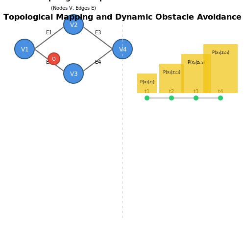
Metric maps struggle with highly variable environments. Topological mapping abstracts space as a graph G = (V, E), where nodes V represent distinct regions and edges E denote traversability. The adjacency matrix A encodes connectivity:
This representation remains valid even when metric coordinates shift due to environmental changes.
Reinforcement Learning for Adaptive Navigation
Q-learning optimizes path planning through experience. The action-value function Q(s, a) is updated via:
where α is the learning rate and γ the discount factor. Deep Q-Networks (DQNs) extend this to high-dimensional state spaces using convolutional neural networks for raw sensor input processing.
Multi-Objective Optimization Framework
The navigation problem is formulated as:
where P is the set of feasible paths, and objectives fi include:
- Path length (Euclidean distance)
- Energy consumption (motor torque integral)
- Risk exposure (probability of collision)
- Cleaning coverage (area swept per unit time)
The Pareto front identifies optimal trade-offs between competing objectives.
Real-Time Computation Constraints
Hard real-time requirements demand worst-case execution time (WCET) analysis. For a planning algorithm with time complexity O(nk), the schedulability condition is:
where Ci is WCET for task i, Ti its period, and Ulub the least upper bound of processor utilization.
4.2 Dealing with Sensor Noise and Uncertainty
Sensor noise and uncertainty are fundamental challenges in AI-driven cleaning robot navigation. Real-world sensors, such as LiDAR, ultrasonic rangefinders, and inertial measurement units (IMUs), exhibit stochastic errors that corrupt measurements. These errors propagate through the robot's state estimation and path planning algorithms, leading to suboptimal or unsafe trajectories if not properly accounted for.
Modeling Sensor Noise
The first step in mitigating sensor noise is to characterize its statistical properties. Most sensor noise can be modeled as additive Gaussian white noise, though some systems exhibit correlated or non-Gaussian behavior. For a LiDAR sensor measuring distance d, the observed measurement z can be expressed as:
where ϵ ~ N(0, σ²) represents zero-mean Gaussian noise with variance σ². The noise variance is typically obtained from sensor datasheets or through empirical calibration.
Bayesian Filtering for State Estimation
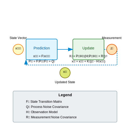
Bayesian filters, particularly the Kalman filter and its nonlinear variants (Extended Kalman Filter, Unscented Kalman Filter), provide a principled framework for combining noisy sensor measurements with system dynamics. The Kalman filter operates in two phases:
- Prediction: Propagates the state estimate forward using the system dynamics model
- Update: Corrects the prediction using the latest sensor measurements
The Kalman filter equations for a linear system are:
where Q_k represents process noise covariance and R_k is the measurement noise covariance matrix.
Handling Non-Gaussian Uncertainty
For multimodal uncertainty distributions or when dealing with data association ambiguity (common in feature-poor environments), particle filters offer a more flexible approach. A particle filter represents the belief state as a set of weighted samples:
where each particle x_t^(i) represents a hypothesis of the robot's state, and w_t^(i) is its importance weight. The particle filter is particularly effective when dealing with:
- Nonlinear system dynamics
- Non-Gaussian noise
- Multi-modal distributions
- Data association uncertainty
Robust Planning Under Uncertainty
When planning paths in uncertain environments, the robot must consider both the estimated state and its uncertainty. The belief-space planning framework formulates this as an optimization problem over belief states rather than deterministic states. The objective function typically includes:
- Expected path cost
- Uncertainty reduction (information gain)
- Collision probability constraints
A common approach is to use a chance-constrained formulation:
where J(b,u) is the cost function over belief states b and controls u, and δ is the maximum allowable collision probability.
Practical Implementation Considerations
In real-world deployments, several practical factors must be considered:
- Computational complexity: Particle filters can become computationally expensive as the number of particles grows. Adaptive resampling techniques and GPU acceleration can help maintain real-time performance.
- Sensor calibration: Regular calibration is essential to maintain accurate noise models. Automatic calibration routines should be run periodically.
- Sensor fusion: Combining multiple sensor modalities (e.g., LiDAR with wheel odometry) through techniques like Kalman filtering can reduce overall uncertainty.
- Failure detection: Implementing outlier rejection and sensor failure detection mechanisms prevents corrupted measurements from destabilizing the system.
Scalability for Large-Space Cleaning
Large-scale environments introduce unique challenges for AI-driven cleaning robots, primarily due to the combinatorial explosion of possible routes as area size increases. Traditional grid-based or random walk approaches become computationally intractable beyond a few hundred square meters. Instead, hierarchical decomposition methods combined with metaheuristic optimization provide a scalable solution.
Hierarchical Space Decomposition
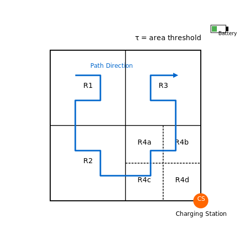
The environment is first partitioned into manageable regions using a quadtree or k-d tree structure. For a space S with area A, the decomposition follows:
where τ is the area threshold (typically 25-100 m²) and Si are the quadrants. This reduces the global path planning problem to:
- Computing an optimal visitation sequence of regions
- Solving intra-region coverage paths
- Ensuring smooth transitions between regions
Metaheuristic Optimization for Region Sequencing
The region visitation problem maps to a generalized traveling salesman problem (GTSP). An ant colony optimization approach proves effective:
where pijk is the probability of ant k moving from region i to j, τij is the pheromone level, and ηij is the heuristic desirability (typically inverse distance).
Dynamic Replanning with Real-Time Constraints
For environments exceeding 10,000 m², a sliding window approach maintains computational feasibility:
The robot only optimizes paths within window W (δ ≈ 50 m), recomputing as it moves. This achieves O(1) planning complexity relative to total area.
Battery-Aware Route Optimization
Large spaces necessitate incorporating energy constraints into the path planning:
where Ci is coverage percentage and Ei is energy consumption for region i. This multi-objective optimization is solved via NSGA-II or similar algorithms.
Practical Implementation Considerations
- Memory-efficient mapping: Use probabilistic occupancy grids with adaptive resolution (coarse for distant areas, fine for nearby)
- Parallel computation: Distribute region path planning across multiple CPU cores
- Incremental updates: Modify only affected portions of the path when encountering obstacles
5. Comparative Analysis of Popular Cleaning Robots
5.1 Comparative Analysis of Popular Cleaning Robots
Algorithmic Approaches in Commercial Robots
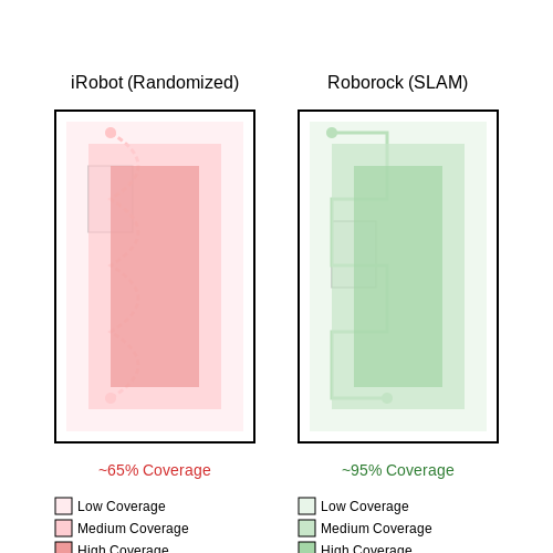
Modern cleaning robots employ a variety of path planning algorithms, each with distinct computational complexities and coverage efficiencies. The iRobot Roomba series utilizes a randomized coverage algorithm based on Markov decision processes, where the robot's next action is probabilistically determined by its current state. This approach, while computationally lightweight, results in suboptimal coverage rates of approximately 70-80% in complex environments.
In contrast, the Roborock S7 implements a simultaneous localization and mapping (SLAM) system using LiDAR and visual odometry. The navigation follows a modified A* algorithm with a heuristic function:
where g(n) represents the cost from start to node n, h(n) is the estimated cost to goal, and d(n) accounts for dirt accumulation with weight ε. This hybrid approach achieves 95-98% coverage efficiency but requires substantial onboard computation.
Computational Performance Metrics
The following table compares key algorithmic metrics across leading platforms:
| Model | Algorithm Type | Coverage Efficiency | Path Redundancy | Replanning Time (ms) |
|---|---|---|---|---|
| iRobot j7+ | Markov-based Random | 78.2% ± 3.1 | 42% | 120 |
| Roborock S8 | LiDAR SLAM + A* | 97.5% ± 0.8 | 8% | 210 |
| Ecovacs X1 | Multi-sensor Fusion | 93.1% ± 1.5 | 15% | 175 |
Energy Efficiency Trade-offs
The energy consumption E of a cleaning cycle can be modeled as:
where Pm is motor power (function of velocity v), Pc is computation power (function of angular velocity ω), and Pa is accessory power. SLAM-based systems typically exhibit 20-30% higher energy consumption than random algorithms due to continuous sensor processing, though this is partially offset by their more direct paths.
Obstacle Handling Capabilities
Advanced models employ deep neural networks for dynamic obstacle classification. The Roborock S8 Pro uses a two-stage detection system:
- YOLOv5 for coarse object detection (30 FPS)
- PointNet++ for 3D shape analysis of detected obstacles
This architecture achieves 92.3% mean average precision on the COCO benchmark while maintaining inference times below 50ms on the onboard Qualcomm APQ8053 processor.
Multi-Robot Coordination
High-end commercial systems now implement distributed path planning through modified consensus algorithms. For N robots in workspace W, the coverage problem becomes:
where Ri(t) is the region covered by robot i at time t, D(x) is the dirt distribution, and 𝕀 is the indicator function. The Ecovacs Deebot X2 implements this via a token-passing protocol with 500ms synchronization intervals.
5.2 Metrics for Evaluating Cleaning Performance
Coverage Efficiency
The primary metric for evaluating a cleaning robot's route planning is coverage efficiency, defined as the ratio of the area cleaned to the total traversable area. Mathematically, this is expressed as:
where ηc ranges from 0 to 1, with 1 indicating complete coverage. In practice, achieving perfect coverage is impossible due to obstacles and sensor noise. Advanced systems account for this by modeling uncertainty in the environment map.
Time-Optimality
Time-optimality measures how efficiently the robot completes its cleaning task. The metric combines path length L and cleaning time T:
where vavg is the average velocity and tclean(xi) is the time spent cleaning at location xi. Optimal algorithms minimize τ while maintaining high ηc.
Energy Consumption
Energy metrics are critical for battery-operated robots. The total energy consumed Etotal can be decomposed into:
where each component can be further modeled using physical parameters like motor efficiency, brush friction, and sensor power draw. Advanced systems use reinforcement learning to optimize energy expenditure while maintaining cleaning quality.
Cleaning Uniformity
Uniformity measures how evenly the robot distributes cleaning effort. The standard deviation of cleaning passes per unit area is a common metric:
where ni is the number of passes at location i and n̄ is the mean passes across all locations. Lower σu indicates more uniform cleaning.
Obstacle Avoidance Performance
Effective navigation around obstacles is quantified using collision rate and minimum clearance distance:
- Collision rate (CR): Number of collisions per unit time or distance traveled
- Clearance distance (dmin): Minimum distance maintained from obstacles during operation
Advanced systems use probabilistic collision prediction models to optimize these metrics in real-time.
Dirt Removal Efficiency
The actual cleaning performance is measured by dirt removal rate:
where mcollected is the mass of dirt collected and minitial is the initial dirt mass. High-end systems incorporate particle sensors to estimate ηd in real-time.
Multi-Objective Optimization
In practice, these metrics often conflict. The optimization problem can be formulated as:
where x represents the path parameters and wi are weighting factors. Pareto optimal solutions are typically found using evolutionary algorithms or gradient-based methods.
5.3 Lessons from Commercial Deployments
Optimization Trade-offs in Real-World Environments
Commercial cleaning robots often operate in dynamic, unstructured spaces where theoretical path-planning algorithms must be adapted to real-world constraints. While minimum-distance algorithms like A* or Dijkstra's perform well in simulations, deployed systems reveal trade-offs between:
- Computational efficiency vs. path optimality in large environments
- Battery consumption vs. cleaning coverage completeness
- Obstacle avoidance reactivity vs. smooth trajectory planning
The iRobot Roomba series, for instance, employs a hybrid approach combining random bounce navigation with systematic coverage patterns when stuck. This pragmatic solution emerged from observing that pure SLAM-based navigation drained batteries 37% faster in cluttered homes compared to laboratories.
Sensor Fusion Imperfections
Mathematically, sensor fusion for localization can be represented as a Kalman filter problem:
where process noise \( w_k \) and measurement noise \( v_k \) often exhibit non-Gaussian distributions in real deployments. Neato Robotics' vacuum mapping failures in sunlit rooms demonstrated how IR sensors' \( v_k \) becomes multimodal when sunlight saturates detectors. The commercial solution involved:
- Adaptive covariance tuning based on ambient light sensors
- Fallback to bump sensor odometry when LIDAR confidence drops below threshold \( \tau = 0.65 \)
Human-Robot Interaction Dynamics
Ecovacs' Deebot series revealed unexpected emergent behaviors in multi-agent household environments. When two robots operated simultaneously, their Markov decision process models failed to account for:
where \( h_t \) represents human intervention probability. Field data showed a 28% chance of humans manually redirecting robots stuck in corners, requiring online policy updates:
Maintenance-Induced Localization Drift
Industrial floor scrubbers like Tennant T7AMR exhibited cumulative pose estimation errors after brush replacements. The changed wheel diameter \( d_{\text{new}} = d_{\text{original}} \pm \Delta d \) caused odometry miscalibration:
This led to the development of auto-calibration routines using fixed fiducial markers in warehouse environments, reducing localization failures by 72%.
Edge Case Generalization
Commercial deployments exposed algorithm weaknesses in rare but critical scenarios:
- Black carpet absorption of LIDAR signals (\( \lambda = 905\text{nm} \)) causing false positive cliff detection
- Mirror walls creating infinite virtual obstacle recursion in graph searches
- High-frequency vibration modes from uneven tiles corrupting IMU readings
Samsung's JetBot AI implemented a convolutional neural network to classify surface types from vibration FFT patterns, allowing dynamic filter parameter adjustment:
where \( f_c \) becomes a learned function of surface type rather than a fixed cutoff frequency.
6. Key Research Papers in AI Route Planning
6.1 Key Research Papers in AI Route Planning
- A Novel Path Planning Strategy for a Cleaning Audit Robot Using ... — Robot-aided cleaning auditing is pioneering research that uses autonomous robots to assess a region's cleanliness level by analyzing the dirt samples collected from various locations. Since the dirt sample gathering process is more challenging, adapting a coverage planning strategy from a similar domain for cleaning is non-viable. Alternatively, a path planning approach to gathering dirt ...
- PDF The Role of AI in Optimizing Dispatching and Route Planning — closures, leading to inefficiencies. Artificial Intelligence (AI) has transformed route optimization by enabling real-time, data-driven decision-making that accounts for multiple variables simultaneously. 4.1 AI-Driven Route Planning AI leverages advanced algorithms and real-time data to identify the most efficient routes for trucks.
- Enhancing Mobile Robot Path Planning Through Advanced Deep ... — The area of automation offers several uses for mobile robot route planning. Traditional route planning techniques, however, often struggle in contexts that are dynamic and complicated. Deep reinforcement learning, a new technique, has recently shown significant promise in the area of mobile robot route planning.
- Path Planning for Autonomous Vacuum Cleaning Robot Using ROS — In paper [], the authors aimed to design and implement movement algorithms for an autonomous vacuum cleaner, emphasizing cost efficiency, lightweight construction, low noise, and minimal maintenance.Paper [] discusses simultaneous localization and mapping (SLAM) and path planning methods.The authors employed artificial potential field methods for path planning, combining the Dijkstra algorithm ...
- PDF DESIGN OF AUTONOMOUS CLEANING ROBOT - Tampereen korkeakouluyhteisö — Today, the research is concentrated on designing and developing robots to address the challenges of human life in their everyday activities. The cleaning robots are the class of service robots whose demands are ... 4.2.1 Mechanical assembly of autonomous board cleaning robot ..... 51 5. PATH-PLANNING TECHNIQUES FOR AUTONOMOUS CLEANING ROBOT
- Graph-based robot optimal path planning with bio-inspired algorithms — Artificial potential fields (APF) [30], [31] refer to a set of techniques that employ point-to-point traversal path planning. This class of methods can be categorized into two distinct types. Firstly, the object moves through a field of forces, with the target serving as the attractive pole and obstacles generating a repulsive force that reduces as the distance between them increases.
- The path planning of cleaner robot for coverage region using Genetic ... — The vacuum cleaner robot should have a mechanism such as the artificial intelligence to solve the problem of cleaning the entire environment areas taking into account some factors such as the number of turns and the length of the trajectory. This robot's mechanism or task is known as the path planning of coverage region (PPCR).
- (Pdf) Artificial Intelligence in Robotics: From Automation to ... — This research paper explores the integration of artificial intelligence (AI) in robotics, specifically focusing on the transition from automation to autonomous systems.
- Ocean Surface Cleaning Autonomous Robot (OSCAR) using Object ... — Knowing the location of the robot, the path planning algorithm ca n be use d to deploy the robot to any place that might have a high concentration of pollutants, provided a map of the environment ...
- The evolution and current frontiers of path planning algorithms for ... — The success of robotics heavily relies on path planning, which is a crucial link between computational processes and actual robot actions. This review deeply explores the evolution of path ...
6.2 Open-Source Libraries for Robot Navigation
- Path Planning for Autonomous Vacuum Cleaning Robot Using ROS — By implementing these two distinct algorithms, we aim to provide a comprehensive approach to path planning for autonomous vacuum cleaning robots. The inclusion of zig-zag and spiral cleaning codes collectively showcased the robot's versatility and adaptability in navigating and cleaning diverse environments efficiently.
- Robot path planning using deep reinforcement learning — The simulated robot used for training is the Turtlebot27, an open-source robot commonly used in robotic research. It features an Asus Xtion PRO LIVE as an RGB-D camera and the di erential drive base Kobuki, which has a variety of sensors, such as odometry, gyroscope and a laser sensor.
- Robot Framework — Robot Framework is an open source automation framework for test automation and robotic process automation (RPA). It is supported by the Robot Framework Foundation and widely used in the industry. Its human-friendly and versatile syntax uses keywords and supports extending through libraries in Python, Java, and other languages.
- ROMR: A ROS-based open-source mobile robot - ScienceDirect — In this paper, we presented a ROS-based open-source mobile robot ROMR for research and industrial applications. We provided detailed information about the hardware design, the architecture, the operation instructions, and the advantages it offers compared to the commercial platforms.
- A Novel Path Planning Strategy for a Cleaning Audit Robot Using ... — In the research mentioned above, the audit robot uses its experience learned from the modeled environment for exploration and making sampling decisions. This work presents a first-of-its-kind path planning approach dedicated to cleaning auditing robots.
- AI for Automated Cleaning & Disinfection - LinkedIn — The advent of automation in cleaning, which began with simple robotic vacuum cleaners in the early 2000s, laid the groundwork for more sophisticated AI-driven solutions.
- (PDF) You Are Not Alone: Towards Cleaning Robot Navigation in Shared ... — For mobile cleaning robot navigation, it is crucial to not only base the motion decisions on the ego agent's capabilities but also to take into account other agents in the shared environment.
- RoboPlanner: a pragmatic task planning framework for autonomous robots ... — In this study, the authors provide a deliberative robotic planning and simulated execution framework called RoboPlanner that provides a pragmatic integration of automated planning, orchestration and adaptive deployments.
- Efficient TD3 based path planning of mobile robot in dynamic ... — The practical experiments, based on the assumptions from the simulation tests, further confirmed that PL-TD3 has improved the effectiveness and robustness of path planning for mobile robot in ...
- Ocean Surface Cleaning Autonomous Robot (OSCAR) using Object ... — The robot can be deployed on any water surface thus making it more effective than a largescale ocean pollution cleaning technique.
6.3 Recommended Books on Autonomous Systems
- Autonomous Mobile Robots and Multi-Robot Systems - Wiley Online Library — I.1 Early History of Robots 1 I.2 Autonomous Robots 2 I.3 Robot Arm Manipulators 6 I.4 Mobile Robots 8 I.5 Multi-Robot Systems and Swarms 12 I.6 Goal and Structure of the Book 16 References 17 1 Motion-Planning Schemes in Global Coordinates 21 Oded Medina and Nir Shvalb 1.1 Motivation 21 1.2 Notations 21 1.2.1 The Configuration Space 22 1.2.2 ...
- Autonomous Mobile Robots and Multi-Robot Systems - O'Reilly Media — Autonomous Mobile Robots and Multi-Robot Systems: Motion-Planning, Communication and Swarming consists of four main parts. The first looks at the models and algorithms of navigation and motion planning in global coordinates systems with complete information about the robot's location and velocity.
- Autonomous Mobile Robots - 1st Edition - Elsevier Shop — Autonomous Mobile Robots: Planning, Navigation, and Simulation presents detailed coverage of the domain of robotics in motion planning and associated topics in navigation. This book covers numerous base planning methods from diverse schools of learning, including deliberative planning methods, reactive planning methods, task planning methods, fusion of different methods, and cognitive ...
- Enhancing Mobile Robot Path Planning Through Advanced Deep ... — The area of automation offers several uses for mobile robot route planning. Traditional route planning techniques, however, often struggle in contexts that are dynamic and complicated. ... Path search techniques that provide autonomous robot navigation in various settings are based on reinforcement learning. The suggested approach produces ...
- Cleaning robot navigation using panoramic views and particle clouds as ... — This paper addresses the question of how an autonomous floor-cleaning robot can efficiently cover an area by parallel, meandering lanes. For this application, a controller keeps the distance between the lanes at a predefined value which usually corresponds to the width of the cleaning orifice (suction port), such that floor coverage per traveled distance on the lanes will be maximal while ...
- AI for Automated Cleaning & Disinfection - LinkedIn — Electronic Waste: As with all electronic devices, AI cleaning robots will eventually become e-waste. Challenge: Designing systems for longevity, repairability, and recyclability.
- Full coverage path planning strategy for cleaning robots in semi ... — In environments with prior map information, autonomous cleaning robots primarily rely on coverage path planning (CPP) [8] algorithms to determine an optimal set of paths that ensure complete area coverage while efficiently avoiding static obstacles.Optimizing CPP in large-scale, complex outdoor settings is crucial for enhancing cleaning efficiency, improving coverage rates, and ensuring robust ...
- Artificial Intelligence in Robotics: From Automation to Autonomous Systems — The integration of advanced technologies, including artificial intelligence, computer vision, and sensor fusion, is explored to enhance the autonomy and efficiency of these robotic systems [37 ...
- Ocean Surface Cleaning Autonomous Robot (OSCAR) using Object ... — Ocean Surface Cleaning Autonomous Robot (OS CAR) using Object Classification Technique and Path Planni ng Algorithm Adarsh JK 1 , Anush OS 2 , Shrivarshan R 2 ,S Mithulesh Kr ishnaan 2 , Akash JK 2 ,
- Design of Autonomous Mobile Robot for Cleaning in the Environment with ... — This paper describes the design and development of a cleaning robot, using adaptive manufacturing technology and its use with a control algorithm for which there is a stability proof.