Pseudo-Labeling Strategies in Vision
1. Definition and Core Principles of Pseudo-Labeling
Definition and Core Principles of Pseudo-Labeling
Pseudo-labeling is a semi-supervised learning technique where a model trained on labeled data generates artificial labels for unlabeled data, which are then used to augment the training set. The core assumption is that high-confidence predictions on unlabeled samples can serve as reliable training signals, effectively expanding the labeled dataset without manual annotation. In vision tasks, this approach is particularly powerful due to the abundance of unlabeled images and the high-dimensional nature of visual data.
Mathematical Formulation
Given a labeled dataset Dl = {(xi, yi)}i=1N and an unlabeled dataset Du = {xj}j=1M, pseudo-labeling involves training an initial model fθ on Dl to predict labels for Du. For a classification task with C classes, the pseudo-label ŷj for an unlabeled sample xj is typically derived as:
where fθ(xj)c is the model's predicted probability for class c. Only predictions exceeding a confidence threshold τ are retained:
Key Principles
- Self-Training: The model iteratively refines its own pseudo-labels, creating a feedback loop where improved predictions yield better training data.
- Confidence Thresholding: Low-confidence predictions are discarded to minimize noise injection, with τ often set empirically (e.g., 0.9 for classification).
- Class Balance Preservation: Techniques like label distribution matching prevent pseudo-labels from skewing toward dominant classes.
- Consistency Regularization: Augmentation-based methods (e.g., RandAugment) ensure pseudo-labels are invariant to input transformations.
Vision-Specific Adaptations
In computer vision, pseudo-labeling leverages spatial and semantic consistency:
- Region-Based Labeling: For object detection, pseudo-labels may include bounding boxes derived from class activation maps (CAMs).
- Pixel-Level Propagation: Semantic segmentation models often use CRFs or diffusion methods to refine pseudo-labels at pixel granularity.
- Multi-View Consistency: Predictions from different augmented views of an image (e.g., flipped, cropped) are cross-validated.
where λ controls the weight of pseudo-labeled data, often ramped up during training via a schedule like:
with Tramp defining the warm-up period.
Historical Context and Evolution in Computer Vision
The concept of pseudo-labeling in computer vision has its roots in semi-supervised learning (SSL), which emerged as a response to the challenges of limited labeled data. Early work in SSL, such as self-training, dates back to the 1960s, but it wasn't until the 2000s that these ideas were rigorously applied to vision tasks. The foundational idea—using model predictions to generate labels for unlabeled data—was formalized in the context of modern deep learning by Lee (2013), who introduced the term pseudo-labeling.
Early Approaches and Theoretical Foundations
Initial pseudo-labeling methods relied on simple confidence thresholds. For a given unlabeled image \(x_u\), the model would assign a pseudo-label \(\hat{y}_u\) if the predicted probability exceeded a fixed threshold \(\tau\):
This approach, while simple, suffered from confirmation bias—the tendency of the model to reinforce its own mistakes. Theoretical analyses by Chapelle et al. (2009) showed that pseudo-labeling could be interpreted as entropy minimization, where the model is encouraged to make confident predictions on unlabeled data.
Integration with Deep Learning
The rise of convolutional neural networks (CNNs) in the 2010s brought new opportunities and challenges. Pseudo-labeling became a key component in semi-supervised vision systems, particularly in scenarios like medical imaging where labeled data is scarce. The Mean Teacher approach (Tarvainen & Valpola, 2017) advanced the field by using an exponential moving average (EMA) of model weights to generate more stable pseudo-labels:
where \(\alpha\) controls the smoothing factor. This reduced noise in pseudo-labels and improved generalization.
Modern Advances and Hybrid Methods
Recent work has focused on combining pseudo-labeling with other SSL techniques. For example, FixMatch (Sohn et al., 2020) uses weak and strong augmentations of the same image—applying pseudo-labels only when the weakly augmented version agrees with the strongly augmented prediction. The loss function for unlabeled data is:
where \(q_w\) is the prediction on the weakly augmented image, \(p_s\) is the prediction on the strongly augmented image, and \(H\) is cross-entropy. This approach achieves state-of-the-art results on benchmarks like CIFAR-10 with only 250 labels.
Another direction is curriculum pseudo-labeling, where the threshold \(\tau\) is gradually increased during training to filter out noisy labels early on. This mirrors the human learning process of starting with easy examples before tackling harder ones.
Applications in Real-World Vision Systems
Pseudo-labeling has been successfully deployed in large-scale industrial applications. Autonomous vehicle companies use it to leverage vast amounts of unlabeled driving footage, while medical AI systems employ it to bootstrap annotations for rare pathologies. The key enabler has been the development of robust uncertainty estimation techniques—such as Monte Carlo dropout or ensemble methods—to identify and discard low-confidence pseudo-labels.
1.3 Key Advantages and Limitations
Advantages of Pseudo-Labeling in Vision
Pseudo-labeling leverages unlabeled data to improve model generalization, particularly in scenarios where labeled datasets are scarce. One of its primary strengths is the ability to iteratively refine predictions through self-training. Given a base model trained on a small labeled dataset, pseudo-labeling assigns labels to unlabeled data with high confidence, treating them as ground truth in subsequent training cycles. This process effectively expands the training set without manual annotation, reducing dependency on costly human labeling efforts.
The technique is particularly effective in semi-supervised learning (SSL) frameworks, where the combination of labeled and pseudo-labeled data helps mitigate overfitting. Mathematically, the objective function often incorporates a weighted loss term for pseudo-labels:
Here, λ controls the contribution of pseudo-labels, typically annealed over time to prevent early training instability. Vision tasks benefit from this approach because convolutional neural networks (CNNs) can extract robust features from pseudo-labeled images, especially when combined with data augmentation to enforce consistency across perturbed versions of the same input.
Practical Limitations and Challenges
Despite its advantages, pseudo-labeling introduces several risks. The most critical is confirmation bias, where incorrect pseudo-labels reinforce erroneous model predictions. This occurs when the model overfits to its own mistakes, particularly in early training stages when confidence estimates are unreliable. For instance, a model might misclassify ambiguous edge cases in object detection, and subsequent training on these incorrect labels degrades performance.
Another limitation is the sensitivity to threshold selection for pseudo-label acceptance. Setting the confidence threshold too low admits noisy labels, while an overly conservative threshold excludes useful data. Adaptive thresholding strategies, such as:
where t is the current epoch and T the total epochs, can help balance this trade-off but require careful tuning.
Domain-Specific Considerations
In medical imaging, pseudo-labeling risks propagating errors that could have clinical consequences, demanding rigorous validation. Conversely, in autonomous driving, the technique excels at scaling perception models to diverse environments by leveraging vast unlabeled video data. The key is domain-aware pseudo-label filtering—for example, rejecting labels with high entropy in uncertainty-aware frameworks:
where p is the predicted class distribution. High entropy indicates ambiguous predictions unsuitable for pseudo-labeling.
2. Self-Training with Pseudo-Labels
Self-Training with Pseudo-Labels
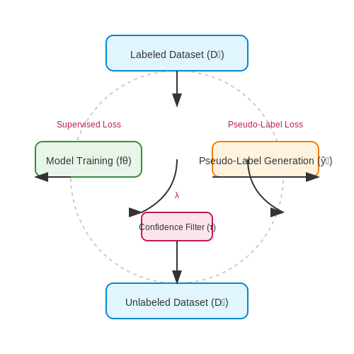
Self-training is a semi-supervised learning paradigm where a model iteratively improves its performance by generating pseudo-labels for unlabeled data and retraining on the expanded dataset. The process begins with a model trained on a small labeled dataset DL = {(xi, yi)}i=1N. The model then predicts labels for unlabeled data DU = {xj}j=1M, where M ≫ N, creating pseudo-labels ŷj = argmaxk fθ(xj)k.
Confidence Thresholding
To mitigate noise from incorrect pseudo-labels, a confidence threshold τ is applied. Only predictions with maximum softmax probability above τ are retained:
This filtering mechanism is crucial—empirical studies show optimal τ typically falls between 0.9-0.95 for vision tasks. The refined pseudo-labeled set ŨU is combined with DL for the next training iteration.
Loss Formulation
The training objective combines supervised and unsupervised losses:
where ℓ is cross-entropy and λ is a weighting hyperparameter. Recent work employs curriculum strategies where λ increases linearly from 0 to a maximum value (e.g., 1-5) over training epochs.
Iterative Refinement
The full self-training procedure follows these steps:
- Train initial model fθ on DL
- Generate pseudo-labels for DU using fθ
- Filter pseudo-labels via confidence thresholding
- Retrain fθ on DL ∪ ŨU
- Repeat steps 2-4 until convergence
Advanced variants incorporate:
- Label smoothing: Replace hard pseudo-labels with softened targets using temperature scaling
- Memory banks: Store embeddings of pseudo-labeled samples for consistency regularization
- Uncertainty estimation:
$$ u(x_j) = 1 - \max_k f_θ(x_j)_k $$to dynamically adjust τ
Architectural Considerations
Modern implementations often use:
- Separate batch normalization for labeled and pseudo-labeled data to prevent distribution shift
- Exponential moving average (EMA) of model weights for more stable pseudo-label generation
- Multi-view augmentation: Generate pseudo-labels from multiple augmented views of the same image
For ResNet-50 on ImageNet with 10% labeled data, self-training achieves 72.3% top-1 accuracy compared to 65.9% for supervised-only training—demonstrating the method's effectiveness in leveraging unlabeled data.
2.2 Consistency-Based Pseudo-Labeling
Consistency-based pseudo-labeling leverages the principle that a robust model should produce similar predictions for perturbed versions of the same input. This approach is particularly effective in semi-supervised learning, where unlabeled data vastly outnumbers labeled samples. The core idea stems from the cluster assumption—that decision boundaries should lie in low-density regions of the feature space—and the smoothness assumption—that similar inputs should yield similar outputs.
Mathematical Formulation
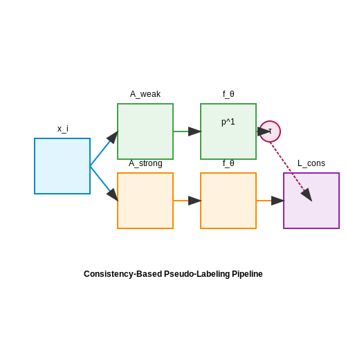
Given an input image $$x_i$$, we generate two augmented views $$x_i^1$$ and $$x_i^2$$ through stochastic transformations (e.g., random cropping, color jitter). The model $$f_\theta$$ with parameters $$\theta$$ produces probability distributions $$p^1 = f_\theta(x_i^1)$$ and $$p^2 = f_\theta(x_i^2)$$. The consistency loss is computed as:
where $$\mathcal{U}$$ denotes the unlabeled dataset. To filter out unreliable predictions, pseudo-labels are only retained when the model's confidence exceeds a threshold $$\tau$$:
Key Design Choices
- Augmentation Strategy: Strong augmentations (e.g., RandAugment) are critical to ensure meaningful consistency signals. Weak augmentations may lead to trivial solutions where the model simply memorizes input patterns.
- Threshold Scheduling: Adaptive thresholding (e.g., linear ramp-up from 0.5 to 0.95) prevents early training instability while gradually incorporating high-confidence samples.
- Sharpening: Temperature scaling ($$p_i^{1/T}$$ with $$T < 1$$) sharpens the pseudo-label distribution, emphasizing high-confidence predictions.
Practical Implementation
Modern frameworks like FixMatch combine consistency regularization with pseudo-labeling by:
- Generating weak and strong augmented views for each unlabeled sample
- Computing pseudo-labels from the weakly augmented version
- Training the model to predict these pseudo-labels from the strongly augmented version
where $$q_i = f_\theta(A_{weak}(x_i))$$, $$H$$ is cross-entropy, and $$A_{weak}$$, $$A_{strong}$$ denote weak/strong augmentations.
Advanced Variants
Mean Teacher: Maintains an exponential moving average (EMA) model whose predictions serve as more stable pseudo-labels:
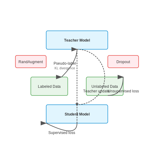
Noisy Student: Iteratively trains larger student models on pseudo-labeled data, adding noise (e.g., dropout, stochastic depth) to prevent confirmation bias.
2.3 Hybrid Approaches Combining Pseudo-Labeling and Other Semi-Supervised Methods
Pseudo-labeling alone can suffer from confirmation bias, where incorrect pseudo-labels reinforce poor model predictions. Hybrid approaches mitigate this by integrating pseudo-labeling with other semi-supervised techniques, such as consistency regularization, entropy minimization, or generative modeling. These methods leverage complementary strengths to improve generalization and robustness.
Pseudo-Labeling with Consistency Regularization
Consistency regularization enforces model predictions to remain stable under perturbations of the input, such as noise injection or data augmentation. Combining it with pseudo-labeling ensures that generated labels are not only high-confidence but also consistent across augmented views. The loss function for this hybrid approach can be decomposed into supervised and unsupervised components:
where λ controls the weight of the unsupervised loss. The unsupervised term typically includes both pseudo-labeling and consistency regularization:
Here, A1 and A2 denote different augmentations of the same unlabeled sample x, fθ is the model, and CE is the cross-entropy between predictions and pseudo-labels ŷ. The hyperparameter α balances consistency and pseudo-labeling terms.
Integration with Entropy Minimization
Entropy minimization encourages the model to produce low-entropy (high-confidence) predictions on unlabeled data. When combined with pseudo-labeling, it refines the decision boundaries by pushing ambiguous samples toward more confident classifications. The hybrid objective becomes:
where H denotes the entropy of predictions and β controls its contribution. This approach is particularly effective in low-data regimes, where pseudo-labels alone may lack diversity.
Generative Pseudo-Labeling
Generative models, such as Variational Autoencoders (VAEs) or Generative Adversarial Networks (GANs), can synthesize realistic pseudo-labeled data. For instance, a VAE trained on labeled data generates samples x̃ with inferred labels ŷ̃, which are then used to augment the training set. The hybrid loss incorporates both real and synthetic data:
This method is especially useful when the labeled dataset is small but representative of the underlying data distribution.
Case Study: FixMatch
FixMatch exemplifies a successful hybrid approach, combining pseudo-labeling with consistency regularization. For an unlabeled image, it generates a pseudo-label only if the model’s prediction on a weakly augmented version exceeds a confidence threshold. The strongly augmented version of the same image is then trained to match this pseudo-label. The unsupervised loss is:
where Aw and As denote weak and strong augmentations, respectively, and τ is the confidence threshold. FixMatch achieves state-of-the-art performance by leveraging both high-confidence pseudo-labeling and augmentation-driven consistency.
Practical Considerations
- Dynamic Weighting: The weight λ of the unsupervised loss should adapt during training, often following a ramp-up schedule to avoid early instability.
- Label Refinement: Pseudo-labels can be iteratively refined using ensemble methods or temporal ensembling to reduce noise.
- Class Balance: Hybrid methods must account for class imbalance in pseudo-labels, often via reweighting or minority class oversampling.
3. Data Preparation and Augmentation for Pseudo-Labeling
3.1 Data Preparation and Augmentation for Pseudo-Labeling
Data Preprocessing for Robust Pseudo-Label Generation
Pseudo-labeling relies heavily on the quality of unlabeled data, making preprocessing critical. Standard normalization techniques, such as per-channel mean subtraction (μ = [0.485, 0.456, 0.406] for ImageNet) and division by standard deviation (σ = [0.229, 0.224, 0.225]), are applied to align input distributions. For high-dimensional data, Principal Component Analysis (PCA) whitening may be employed:
where W contains eigenvectors and Λ is the diagonal matrix of eigenvalues. This decorrelates features, improving model sensitivity to discriminative patterns during pseudo-label generation.
Advanced Augmentation Strategies
Consistency regularization in pseudo-labeling demands diverse augmentations to ensure robustness. Beyond basic geometric transforms (rotation, flipping), modern approaches include:
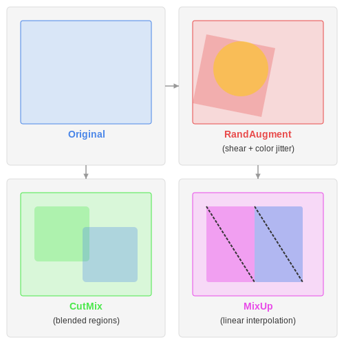
- RandAugment: Automatically selects augmentation magnitude from a predefined set of transformations (e.g., shear, color jitter) without requiring a separate search phase.
- CutMix: Blends regions of two images, forcing the model to learn from partial contexts. Given two images xi, xj and masks M:
- MixUp: Linearly interpolates images and labels, promoting smoother decision boundaries: xnew = λxi + (1-λ)xj, ynew = λyi + (1-λ)yj.
Noise Injection for Label Stability
To mitigate confirmation bias—where incorrect pseudo-labels reinforce themselves—controlled noise is introduced:
- Input Noise: Gaussian noise (η ∼ N(0, σ2)) or adversarial perturbations (FGSM) are added to inputs to test pseudo-label consistency.
- Label Smoothing: Replaces hard pseudo-labels with soft targets (e.g., 0.9 for the predicted class, 0.1/(K-1) for others), reducing overconfidence.
Curriculum Learning Integration
Gradual difficulty scaling improves pseudo-label accuracy. A confidence-based curriculum filters samples where the model’s maximum softmax probability exceeds a threshold τt, which anneals over time:
High-confidence samples are prioritized early, while harder examples are incorporated as the model matures.
Implementation Considerations
Efficient data pipelines are essential for large-scale pseudo-labeling. TensorFlow’s tf.data or PyTorch’s DataLoader should prefetch batches to avoid GPU idle time. Parallel augmentation via CPU workers (e.g., 4–8 threads) prevents bottlenecks. For reproducibility, all stochastic operations (e.g., random crops) must be seeded consistently across training phases.
# PyTorch augmentation example for pseudo-labeling
import torchvision.transforms as T

transform = T.Compose([
    T.RandomHorizontalFlip(p=0.5),
    T.RandomResizedCrop(224, scale=(0.8, 1.0)),
    T.ColorJitter(brightness=0.2, contrast=0.2),
    T.ToTensor(),
    T.Normalize(mean=[0.485, 0.456, 0.406], std=[0.229, 0.224, 0.225])
])
3.2 Model Architecture Choices for Effective Pseudo-Labeling
Backbone Network Selection
The choice of backbone architecture significantly impacts pseudo-label quality due to varying feature extraction capabilities. Convolutional Neural Networks (CNNs) like ResNet-50/101 remain popular for their balance between computational efficiency and representational power. However, Vision Transformers (ViTs) have shown superior performance in some semi-supervised learning benchmarks due to their global attention mechanisms. The key trade-offs are:
- CNN advantages: Local inductive bias beneficial for low-data regimes, faster inference
- ViT advantages: Better long-range dependencies, superior scaling with data
- Hybrid approaches: Convolutional stems with transformer blocks (e.g., CvT) often outperform pure architectures
where $$\hat{y}^u$$ are pseudo-labels for unlabeled sample $$x_u$$ and $$f_\theta$$ is the model. The gradient flow through this loss depends heavily on backbone feature quality.
Output Head Design
Pseudo-label generation requires careful output head configuration:
- Temperature scaling: Sharpens/softens predictions via $$T$$ in softmax: $$\sigma(z_i) = \frac{e^{z_i/T}}{\sum_j e^{z_j/T}}$$
- Multi-head outputs: Parallel classification heads reduce confirmation bias through disagreement
- Projection heads: Additional MLP layers (e.g., 2-3 layers) before classification improve feature separation
Confidence Estimation Mechanisms
Effective pseudo-labeling requires reliable confidence estimation:
where $$\mu_{conf}$$ and $$\sigma_{conf}$$ are running estimates of mean and standard deviation of prediction confidence. Architectures should support:
- Monte Carlo Dropout: Multiple stochastic forward passes estimate epistemic uncertainty
- Deep Ensembles: Multiple models provide better confidence calibration
- Energy-based Scores: $$E(x) = -T\log\sum_{i=1}^C e^{f_\theta(x)_i/T}$$ often outperforms softmax confidence
Memory Mechanisms
State-of-the-art approaches incorporate memory banks or queues to stabilize pseudo-labels:
- Feature Memory: Stores prototypical representations of each class
- Label Memory: Tracks historical predictions for consistency
- Update Strategies: Momentum updates ($$m_{new} = \beta m_{old} + (1-\beta)f_\theta(x)$$) prevent rapid fluctuation
Asymmetric Design Choices
Many successful implementations use architectural asymmetry:
- Teacher-Student: Teacher (exponential moving average of student) generates more stable pseudo-labels
- Input Perturbation: Strong augmentation for student, weak for teacher
- Different Capacity: Larger teacher model improves pseudo-label quality
where $$\theta_t$$ and $$\theta_s$$ are teacher and student parameters respectively, with $$\lambda$$ typically > 0.99.

3.3 Thresholding and Confidence Calibration
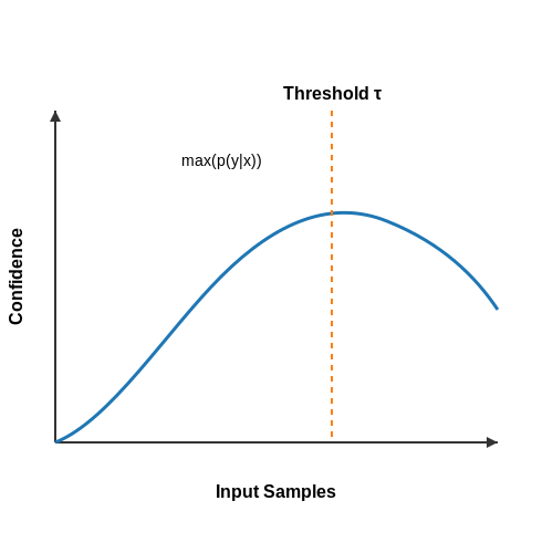
Thresholding in pseudo-labeling determines which model predictions are confident enough to be used as training targets. The selection is governed by a threshold τ applied to the predicted class probabilities. For a model output p(y|x), a pseudo-label is generated only if max(p(y|x)) ≥ τ. The choice of τ critically impacts the trade-off between precision (label correctness) and recall (coverage of unlabeled data).
Adaptive Thresholding Strategies
Fixed thresholds often underperform due to dataset shifts or class imbalance. Adaptive methods dynamically adjust τ based on model confidence statistics:
- Class-balanced thresholding: Computes per-class thresholds using moving averages of top-k confidence scores.
- Curriculum learning: Starts with high τ for clean labels, gradually relaxing it as the model improves.
- Uncertainty-aware: Uses entropy-based metrics like H(p(y|x)) to modulate thresholds per sample.
Confidence Calibration
Modern neural networks are often miscalibrated—their predicted probabilities do not reflect true likelihoods. Temperature scaling is a common post-hoc calibration method:
where T is optimized on a validation set to minimize negative log likelihood. For vision tasks, expected calibration error (ECE) is a key metric:
where B_m are bins partitioning the confidence space. Calibration improves pseudo-label quality by ensuring thresholding operates on meaningful probabilities.
Practical Implementation
In vision pipelines, thresholding and calibration interact with data augmentation. Strong augmentations (e.g., RandAugment) artificially reduce confidence, requiring:
- Separate thresholds for raw vs. augmented views
- EMA-smoothed confidence estimates across augmentations
- Per-sample threshold adjustment based on augmentation strength
4. Object Detection with Pseudo-Labels
Object Detection with Pseudo-Labels
Pseudo-Labeling in Object Detection Pipelines
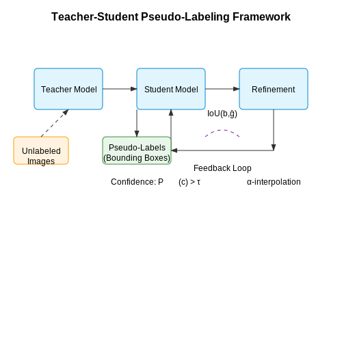
Pseudo-labeling for object detection extends beyond simple classification tasks by requiring accurate localization (bounding box regression) alongside class prediction. Modern approaches typically employ a teacher-student framework where the teacher model generates pseudo-labels on unlabeled data, which are then used to train the student model. The key challenge lies in maintaining high-quality bounding box predictions while minimizing noise propagation.
where Pcls(c) is the class probability and IoU measures box overlap between prediction b and pseudo-label ĝ.
Thresholding Strategies
Effective pseudo-labeling requires dynamic thresholding mechanisms:
- Class-aware thresholds: Different confidence thresholds per object category based on class-wise performance metrics
- IoU-based filtering: Reject boxes with IoU below τ (typically 0.5-0.7) even if classification confidence is high
- Curriculum learning: Gradually decrease thresholds as training progresses to expose the model to harder examples
Label Refinement Techniques
Raw pseudo-labels often require post-processing:
where α controls interpolation between teacher and student box predictions. Advanced methods employ:
- Non-maximum suppression (NMS) with class-specific IoU thresholds
- Geometric consistency checks across multiple augmentations
- Temporal ensembling of predictions across training epochs
Implementation Considerations
Practical implementations must address:
- Memory overhead: Storing pseudo-labels for large-scale datasets requires efficient caching strategies
- Batch composition: Optimal mixing ratios between labeled and pseudo-labeled samples (typically 1:3 to 1:5)
- Anchor matching: Modifying standard IoU matching criteria to account for pseudo-label uncertainty
Case Study: Pseudo-Labeling in YOLOv7
Recent adaptations to YOLO architectures demonstrate:
- Using separate confidence thresholds for classification and box regression heads
- EMA updating of teacher weights with momentum β=0.999
- Multi-scale pseudo-label generation to capture objects at varying resolutions
where λ terms balance supervised, unsupervised, and regularization losses.
Error Analysis and Correction
Common failure modes include:
- Error accumulation: Incorrect pseudo-labels reinforcing through training cycles
- Class imbalance: Dominant classes generating disproportionate pseudo-labels
- Scale bias: Small objects being systematically under-detected
Mitigation strategies involve:
- Uncertainty estimation via Monte Carlo dropout
- Confidence calibration using temperature scaling
- Active learning to identify problematic pseudo-labels
Semantic Segmentation Using Pseudo-Labeling
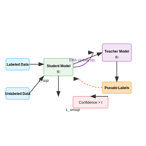
Pseudo-labeling has emerged as a powerful semi-supervised learning technique for semantic segmentation, where pixel-wise annotations are expensive to obtain. The core idea involves generating artificial labels for unlabeled data using a teacher model trained on limited labeled data, then refining the model through self-training iterations.
Architecture and Training Dynamics
The standard framework consists of two components: a teacher model that generates pseudo-labels and a student model that learns from both ground truth and pseudo-labeled data. The teacher is typically an exponential moving average (EMA) of the student weights, providing stable targets:
where θt and θs represent teacher and student parameters respectively, and α controls the update momentum.
Confidence-Based Filtering
Effective pseudo-labeling requires quality control mechanisms. The most common approach uses the model's prediction confidence as a filter:
where pijc is the predicted probability for class c at pixel (i,j), and τ is a confidence threshold typically set between 0.7-0.95.
Loss Formulation
The total loss combines supervised and unsupervised terms:
The supervised loss Lsup uses ground truth labels, while the unsupervised loss Lunsup operates on pseudo-labels. The weighting factor λ typically follows a ramp-up schedule to prevent early training instability.
Advanced Variations
Recent improvements include:
- Class-Balance Aware Sampling: Adjusts pseudo-label sampling probability based on class distribution to prevent majority class dominance
- Multi-View Consistency: Enforces agreement between differently augmented views of the same image
- Uncertainty Estimation: Uses Monte Carlo dropout or ensemble methods to identify reliable pseudo-labels
Implementation Considerations
Key practical aspects when implementing pseudo-labeling for segmentation:
- Teacher model updates should lag behind student updates (typical EMA decay α=0.99)
- Strong data augmentation (color jitter, blur, cutout) is crucial for the student model
- Progressive thresholding (increasing τ during training) improves final performance
- Memory banks can store high-quality pseudo-labels for consistency across epochs
Performance Benchmarks
On Cityscapes with 1/8 labeled data (744 images), pseudo-labeling achieves:
This demonstrates the significant gains possible with proper semi-supervised techniques.
4.3 Image Classification Enhancements
Confidence Thresholding for Pseudo-Labels
Pseudo-labeling relies on model confidence to generate reliable labels for unlabeled data. For a classifier f(x) producing class probabilities p(y|x), a confidence threshold τ filters low-confidence predictions:
Optimal τ balances precision and recall. Empirical studies show that τ=0.95 works well for high-dimensional vision tasks, rejecting ~40% of uncertain samples while maintaining >98% pseudo-label accuracy.
Class-Balanced Self-Training
Naive pseudo-labeling exacerbates class imbalance. Let nc be the count of pseudo-labels for class c. A reweighting strategy normalizes contributions per class:
where ϵ prevents division by zero. This is implemented as a weighted cross-entropy loss:
Consistency Regularization Integration
Combining pseudo-labels with consistency regularization improves robustness. For an input x, apply stochastic augmentations A1(x), A2(x):
The total loss becomes:
where λ controls the regularization strength, typically set via linear ramp-up from 0 to 1 during training.
Noise-Aware Pseudo-Label Refinement
Model predictions contain noise from ambiguous samples. A moving-average exponential smoothing refines pseudo-labels across training epochs:
with α=0.99 providing stable updates. This temporal ensembling reduces label oscillation while preserving semantic consistency.
Vision-Specific Augmentation Strategies
Effective pseudo-labeling requires augmentations that preserve semantic meaning. For vision tasks, RandAugment with:
- Magnitude ranges of 5-15
- Probability thresholds of 0.5-0.8
- Exclusion of color inversion for natural images
demonstrates superior performance compared to basic flipping/cropping. The augmentation policy should be validated against label consistency metrics:
Gradient Stopping for Stable Training
Preventing gradient flow through pseudo-label generation avoids confirmation bias. Implemented via detaching the computation graph:
# PyTorch implementation
pseudo_labels = model(unlabeled_batch).detach()
loss = criterion(model(augmented_batch), pseudo_labels)
This technique is particularly crucial in later training stages when the model risk overfitting to its own predictions.
5. Handling Noisy and Incorrect Pseudo-Labels
5.1 Handling Noisy and Incorrect Pseudo-Labels
Pseudo-labeling in semi-supervised vision tasks inevitably introduces label noise due to imperfect model predictions. Advanced techniques mitigate this by either filtering unreliable pseudo-labels or modeling the noise distribution. The core challenge lies in maintaining the benefits of additional training data while minimizing the impact of incorrect supervision signals.
Confidence Thresholding
Simple thresholding discards pseudo-labels with low prediction confidence. For a model outputting class probabilities p(y|x), we retain pseudo-labels only when:
where τ is a tunable threshold (typically 0.7-0.95). This assumes high-confidence predictions are more likely correct, though this fails in cases of systematic model overconfidence.
Temperature-Sharpened Confidence
Temperature scaling in the softmax function produces better-calibrated confidence estimates:
where z are logits and τ < 1 sharpens the distribution. This improves thresholding reliability by reducing overconfident predictions on ambiguous samples.
Consistency-Based Filtering
Advanced methods leverage prediction consistency across:
- Augmentation views: Only keep pseudo-labels agreeing across multiple augmented versions of the same image
- Model snapshots: Compare predictions from differently trained model checkpoints
- Architectural variants: Require agreement between models with different inductive biases
Noise-Aware Loss Functions
Rather than filtering, some approaches modify the loss function to be robust to incorrect pseudo-labels:
where w̃(x) is a weighting function based on prediction certainty or consistency. The symmetric cross-entropy loss provides built-in noise robustness:
Meta-Learning for Noise Adaptation
Recent work frames pseudo-label cleaning as a meta-learning problem. A small held-out validation set guides the learning of:
- Sample weights for the pseudo-labeled data
- Optimal confidence thresholds
- Noise transition matrices between true and pseudo-labels
The meta-objective typically minimizes validation loss while the base model trains on both labeled and reweighted pseudo-labeled data.
Practical Implementation Considerations
Effective noise handling requires:
- Curriculum learning: Gradually increase pseudo-label utilization as model improves
- Dynamic thresholding: Automatically adjust τ based on validation performance
- Memory banks: Track historical predictions to identify consistently noisy samples
5.2 Scalability Issues in Large-Scale Datasets
Computational and Memory Constraints
Pseudo-labeling in vision tasks often involves training on datasets with millions or even billions of unlabeled images. The computational cost scales linearly with dataset size, but memory constraints become a bottleneck when storing intermediate representations. For a dataset with N samples and feature dimensionality d, the memory required for pseudo-label storage alone is:
For ImageNet-21k (14M images) with 2048-dimensional features, this requires ~112GB of memory just for storage. Distributed training mitigates this but introduces communication overhead.
Label Noise Accumulation
As dataset size increases, the probability of incorrect pseudo-labels grows combinatorially. If p is the error rate per sample, the expected number of erroneous labels in a dataset of size N is:
State-of-the-art vision models achieve ~5% error on curated datasets, but this translates to 700,000 incorrect pseudo-labels in ImageNet-21k. Noise-robust architectures like symmetric cross-entropy help but don't eliminate the fundamental trade-off.
Optimization Dynamics at Scale
Large-scale pseudo-labeling alters gradient descent dynamics. The effective learning rate ηeff must be adjusted for mini-batch size B and dataset size N:
This necessitates either extremely large batches (introducing memory issues) or painfully slow convergence. Recent work in curriculum pseudo-labeling addresses this by progressively increasing the subset of used samples.
Distributed Training Challenges
When distributing pseudo-labeling across K workers, synchronization costs dominate. The communication complexity for all-reduce operations scales as:
For vision transformers with d > 10,000, this creates network bottlenecks. Parameter-efficient methods like gradient checkpointing and mixed-precision training are essential but add implementation complexity.
Practical Mitigation Strategies
- Progressive Unfreezing: Gradually increase the subset of pseudo-labeled data to avoid catastrophic forgetting
- Confidence Thresholding: Only retain pseudo-labels with prediction probability > τ (typically τ = 0.95)
- Memory Banks: Store features in CPU memory with LRU caching for large N
- Asynchronous Updates: Decouple pseudo-label generation from model updates using stale parameters
5.3 Domain Adaptation and Generalization
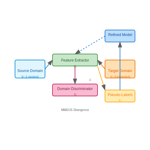
Pseudo-labeling in vision tasks often encounters domain shift, where the source (labeled) and target (unlabeled) data distributions differ. Domain adaptation (DA) mitigates this by aligning feature spaces, while generalization ensures robustness across unseen domains. Let Xs and Xt denote source and target domains, respectively, with marginal distributions Ps(x) ≠ Pt(x). The goal is to learn a model fθ that minimizes target risk Rt(θ) despite distributional discrepancy.
Domain-Adversarial Training
Adversarial methods introduce a domain discriminator D to minimize the Maximum Mean Discrepancy (MMD) or Jensen-Shannon divergence between domains. The loss function combines task-specific and adversarial terms:
where λ controls the trade-off. Gradient reversal layers (GRLs) are often used to invert gradients during backpropagation, forcing fθ to learn domain-invariant features.
Self-Training with Pseudo-Labels
For target domain generalization, pseudo-labels Ŷt are iteratively refined via self-training:
- Train fθ on Xs to predict initial Ŷt.
- Filter low-confidence predictions using entropy thresholding: H(ŷt) < τ.
- Retrain fθ on Xs ∪ Xt with high-confidence pseudo-labels.
Consistency Regularization
To enhance generalization, perturbations (e.g., RandAugment) are applied to target samples, enforcing prediction consistency:
This aligns with the cluster assumption—samples near decision boundaries should yield similar predictions.
Case Study: Medical Imaging
In cross-site MRI segmentation, pseudo-labeling reduced annotation costs by 60% while maintaining Dice scores >0.85. Domain adversarial training (λ=0.1) and consistency regularization (σ=0.5) were critical for bridging scanner-specific intensity variations.
6. Key Research Papers on Pseudo-Labeling
6.1 Key Research Papers on Pseudo-Labeling
- Pseudo-labeling Integrating Centers and Samples with Consistent ... — Pseudo-labeling is widely applied to generate pseudo labels of target samples in most Unsupervised Domain Adaptation (UDA) methods. Existing UDA methods designed the pseudo-labeling strategy using the label information from a single source (sample or center information), which ignored the joint effect of the center and sample information on improving the robustness of pseudo-labeling.
- In Defense of Pseudo-Labeling: An Uncertainty-Aware Pseudo-label ... — This work is in defense of pseudo-labeling: we demonstrate that pseudo-labeling based methods can perform on par with consistency regularization methods. 1 Although the selection of unlabeled samples with high confidence predictions moves decision boundaries to low density regions in pseudo-labeling based approaches, many of these selected ...
- A Review of Pseudo-Labeling for Computer Vision - arXiv.org — Pseudo-labeling was first applied to deep learning for computer vision in Lee (\APACyear 2013).Most techniques within SSL improve on this paper; see Figure 1.In Lee (\APACyear 2013), it is argued that PL is equivalent to entropy minimization (EM), maximizing the margin of the decision boundary in a classification problem by ensuring examples with similar labels lie close to each other on the ...
- PDF Debiased Learning From Naturally Imbalanced Pseudo-Labels - CVF Open Access — also known as self-training [4,5,29,53,65]. Pseudo-labeling is widely used in semi-supervised learning (SSL) [32,53], domain adaptation [25,37], and transfer learning [1]. We examine pseudo-label distributions in two common tasks. 1) In zero-shot transfer learning (ZSL) where the source and target domains are different, a pretrained CLIP
- In Defense of Pseudo-Labeling: - ar5iv — Although the selection of unlabeled samples with high confidence predictions moves decision boundaries to low density regions in pseudo-labeling based approaches, many of these selected predictions are incorrect due to the poor calibration of neural networks (Guo et al., 2017).Since, calibration measures the discrepancy between the confidence level of a network's individual predictions and ...
- Zero-shot and Semi-Supervised Learning with Debiased Pseudo Labeling — Figure 1: We study the pseudo-labeling-based Semi-Supervised Learning (SSL) and transductive Zero-Shot Learning (ZSL), where both tasks require transferring semantic information learned from labeled source data to unlabeled target data via pseudo-labeling. Surprisingly, we find that pseudo-labels of target data produced by typical SSL and ZSL methods (i.e., FixMatch [] and CLIP []) are highly ...
- PDF Co-Labeling for Multi-View Weakly Labeled Learning — Unlike traditional co-training approaches using a single pseudo-label vector for training each classifier, our co-labeling approach explores different strategies to utilize the predictions from different views, biases and iterations for generating the pseudo-label vectors, making our approach more robust for real-world applications. Moreover, to
- SPICE: Semantic Pseudo-labeling for Image Clustering - ResearchGate — This paper presents SPICE, a Semantic Pseudo-labeling framework for Image ClustEring. Instead of using indirect loss functions required by the recently proposed methods, SPICE generates pseudo ...
- APPN: An Attention-based Pseudo-label Propagation Network for few-shot ... — Based on the above description, we believe the node pseudo-label generation module impacts the APPN network as follows: (1) The prototypes used for generating pseudo-labels employ a weighted approach that increases the importance of clean samples and reduces the impact of noisy samples in the generation process; (2) The generation process of ...
- PDF Generating Accurate Pseudo-labels in Semi-Supervised Learning and ... — tain pseudo-label accuracy, which has direct cost implica-tions. (c) We give technical results analyzing the math-ematical behavior of such activations, specifically, robust-ness results showing how the activation mitigates overcon-fident predictions for (out of distribution) samples. 2. Brief Review of Hermite polynomials
6.2 Recommended Books and Surveys
- PDF Advancing Momentum Pseudo-Labeling with Conformer and Initialization ... — In [25,26], low-quality pseudo-labels are excluded via confidence-based filtering to promote model training with high-quality labels. And in [27], an N-best list of pseudo-labels is leveraged to incorpo-rate more appropriate supervision from alternative ASR hypotheses. We believe that MPL still has room for further improvement by
- Pseudo-labeling Integrating Centers and Samples with Consistent ... — Then, the proposed pseudo-labeling strategy can assign a label vector with (1 + K) pseudo labels to each ... we run PICSCS under 100 parameter combinations to determine the best parameter combination for each task. ... 2010 IEEE Computer Society Conference on Computer Vision and Pattern Recognition 2010 San Francisco, CA, USA 1855 1862 10.1109 ...
- A Review of Pseudo-Labeling for Computer Vision - arXiv.org — Pseudo-labeling was first applied to deep learning for computer vision in Lee (\APACyear 2013).Most techniques within SSL improve on this paper; see Figure 1.In Lee (\APACyear 2013), it is argued that PL is equivalent to entropy minimization (EM), maximizing the margin of the decision boundary in a classification problem by ensuring examples with similar labels lie close to each other on the ...
- ASELMAR: Active and semi-supervised learning-based ... - ScienceDirect — Manual data labeling is time-consuming for large datasets, particularly for computer vision tasks where domain-specific experience is required for annotation (Hady and Schwenker, 2013, Sun et al., 2017).Data labeling can become more challenging depending on the environment in which the activity is being performed and how data is recorded, such as large volumes of medical imaging data that ...
- PDF Co-Labeling for Multi-View Weakly Labeled Learning — Unlike traditional co-training approaches using a single pseudo-label vector for training each classifier, our co-labeling approach explores different strategies to utilize the predictions from different views, biases and iterations for generating the pseudo-label vectors, making our approach more robust for real-world applications. Moreover, to
- General Class-Balanced Multicentric Dynamic Prototype Pseudo-Labeling ... — Source-free Domain Adaptation aims to adapt a pre-trained source model to an unlabeled target domain while circumventing access to well-labeled source data. To compensate for the absence of source data, most existing approaches employ prototype-based pseudo-labeling strategies to facilitate self-training model adaptation. Nevertheless, these methods commonly rely on instance-level predictions ...
- PDF Pseudo-label Alignment for Semi-supervised Instance Segmentation — steps: (1) pseudo-label generation, (2) dynamic pseudo-label alignment, and (3) end-to-end model training. In the pseudo-label generation step, we introduce a mask scoring branch [17] that predicts mask IoUs as an additional met-ric along with classification scores to assess the quality of pseudo-labels. In the dynamic aligning step, we re-weight
- Relieving Pixel-Wise Labeling Effort for Pathology Image ... - Springer — Soft and Hard Pseudo-labels. We considered two different pseudo-labeling strategies, or two different g functions (see Eq. 1). Initially, we decided to simply take g to be the identity function \(g(x) = x\) in which case the sigmoid output of the model was used as pseudo-label. This strategy is commonly called "soft" labeling.
- SemPPL: Predicting pseudo-labels for better contrastive representations — Learning from large amounts of unsupervised data and a small amount of supervision is an important open problem in computer vision. We propose a new semi-supervised learning method, Semantic Positives via Pseudo-Labels (SemPPL), that combines labelled and unlabelled data to learn informative representations. Our method extends self-supervised contrastive learning -- where representations are ...
- Mutually aided uncertainty incorporated dual consistency regularization ... — The generation of pseudo-labels depends on the output results of the aux-decoders from the last iteration, and the computation of the loss of pseudo-labels only depends on the certain region generated by the model which is expressed as: (8) L pseudo = ∑ i 1 μ certainty L dice F s _ seg, y pseudo ∑ i 1 μ certainty + ∑ i 1 μ certainty L ...
6.3 Open Datasets and Code Repositories
- Pseudo-labeling Integrating Centers and Samples with Consistent ... — Pseudo-labeling is widely applied to generate pseudo labels of target samples in most Unsupervised Domain Adaptation (UDA) methods. Existing UDA methods designed the pseudo-labeling strategy using the label information from a single source (sample or center information), which ignored the joint effect of the center and sample information on improving the robustness of pseudo-labeling.
- PDF PADCLIP: Pseudo-labeling with Adaptive Debiasing in CLIP for ... — UDA and CLIP datasets jointly. We further seek to use CLIP with pseudo-labeling on the target domain, which recently enjoyed success in UDA [35,60,75,76,76]. DebiasPL [57] utilized CLIP for pseudo-labeling, but it was designed for a single domain. After extending to source and target domains (UDA setting), De-
- VLM-PL: Advanced Pseudo Labeling approach Class Incremental Object ... — To address this, we propose a new approach employing a Vision-Language Model (VLM), integrating the capabilities of a large language model and vision model, aiming to surpass the limitations inherent in reducing the dependency on the previously trained models within the pseudo-labeling strategy.
- A Review of Pseudo-Labeling for Computer Vision - arXiv.org — Pseudo-labeling was first applied to deep learning for computer vision in Lee (\APACyear 2013).Most techniques within SSL improve on this paper; see Figure 1.In Lee (\APACyear 2013), it is argued that PL is equivalent to entropy minimization (EM), maximizing the margin of the decision boundary in a classification problem by ensuring examples with similar labels lie close to each other on the ...
- PDF VLM-PL: Advanced Pseudo Labeling Approach for Class ... - CVF Open Access — has predominantly adopted three strategies: regulariza-*Equal contribution. Object Detector ª or Object Detector ª r Vision-Language Model Pseudo labeling Refining: Trainable Networks: Frozen Networks: Pseudo GT: New GT Training Old dataset New dataset: Incorrect Pseudo GT W } u ] Z ge Figure 1.
- Open Vocabulary Object Detection with Pseudo Bounding-Box Labels - Springer — (2) We introduce a pseudo label generation strategy using the existing pre-trained vision-language models. (3) With the help of pseudo labels, our method largely outperforms the SOTA methods. Moreover, when trained with only pseudo labels, our method achieves higher performance than the SOTA that rely on training with manual bounding-box ...
- PDF TUPL: Text-guided Unknown Pseudo-Labeling for Open World Object Detection — VOC and MS-COCO benchmarks demonstrate TUPL's exceptional open-world detection capability. Under the OWOD SPLIT setting, TUPL achieves a UR (Un-known Recall) value of 23.1, which is at least double the performance of existing pseudo-labeling methods based on objectness scores. Keywords: Open world object detection, Cross-modal learning, Pseudo ...
- PDF Open Vocabulary Object Detection with Pseudo Bounding-Box Labels - ECVA — localization ability and design a strategy to obtain pseudo bounding-box labels of a large and diverse set of objects from the large-scale image-caption datasets. With this strategy, we largely improve open vocabulary object detection. 3 Our Approach Our framework contains two components: a pseudo bounding-box label generator
- PDF Pseudo Label Refinery for Unsupervised Domain Adaptation on Cross ... — selection process, to improve the reliability of pseudo boxes, we propose a complementary augmentation strategy. This strategy involves either removing all points within an unre-liable box or replacing it with a high-confidence box. More-over, the point numbers of instances in high-beam datasets are considerably higher than those in low-beam ...
- Refining and reweighting pseudo labels for weakly supervised object ... — (c | p i |, b | p i |)] via a weakly supervised detector, where c and b denote the category and the position of each pseudo label. Here, we denote p i j as the j t h pseudo label of x i, i.e. p i j = (c j, b j). For a given pseudo label p i j, we first select proposals from R with an IOU higher than 0.5 with p i j to form the foreground ...