Dreaming Agents: Offline Simulation and Planning
1. Defining Dreaming Agents in AI
1.1 Defining Dreaming Agents in AI
Dreaming agents in artificial intelligence refer to systems capable of simulating hypothetical scenarios—dreams—without direct interaction with the real environment. These agents leverage offline data, generative models, and reinforcement learning to explore possible futures, optimize policies, and improve decision-making under uncertainty. The concept draws inspiration from cognitive science, where mental simulation plays a key role in human planning and creativity.
Core Components of Dreaming Agents
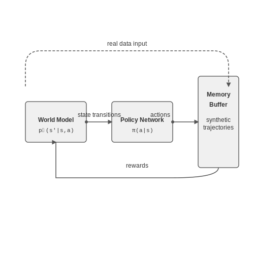
A dreaming agent typically consists of three interconnected modules:
- World Model: A learned or pre-defined simulator that generates plausible state transitions and rewards. Often implemented as a neural network trained on historical data (e.g., a variational autoencoder or diffusion model).
- Policy Network: Maps states to actions, refined through simulated trajectories. Uses algorithms like Proximal Policy Optimization (PPO) or Soft Actor-Critic (SAC).
- Memory Buffer: Stores synthetic experiences for offline training, enabling iterative policy improvement without real-world exploration.
Mathematical Formulation
Given a Markov Decision Process (MDP) with states s, actions a, and rewards r, a dreaming agent learns a world model p̂(s'|s, a) approximating the true dynamics p(s'|s, a). The agent optimizes its policy π(a|s) by maximizing the expected return in the simulated environment:
where γ is the discount factor. The world model is trained to minimize the Kullback-Leibler divergence between real and synthetic state transitions:
Applications and Case Studies
Dreaming agents excel in domains where real-world exploration is costly or dangerous, such as:
- Autonomous Driving: Simulation of rare traffic scenarios to improve collision avoidance policies.
- Healthcare: Predicting patient outcomes under hypothetical treatment plans using electronic health records.
- Robotics: Training robotic manipulators in synthetic environments before hardware deployment.
For example, DeepMind's DreamerV3 achieves superhuman performance in Atari games by learning entirely from imagined rollouts, demonstrating sample efficiency gains of 10–100× over model-free methods.
Limitations and Open Challenges
Key unresolved issues include:
- Model Bias: Discrepancies between simulated and real dynamics can lead to catastrophic failures.
- Long-Horizon Planning: Credit assignment over extended dream sequences remains computationally intensive.
- Non-Stationarity: Adapting world models to environments with shifting dynamics (e.g., weather changes in autonomous systems).
Recent advances in hierarchical world models and uncertainty quantification aim to address these limitations, as seen in architectures like PlaNet and I2A.
Core Principles of Offline Simulation
Model-Based Dynamics Approximation
Offline simulation relies on approximating environment dynamics using learned models, typically represented as Markov Decision Processes (MDPs). The transition dynamics T(s'|s,a) and reward function R(s,a) are estimated from static datasets D = {(si, ai, s'i, ri)}. For continuous state spaces, Gaussian Processes or Neural Networks parameterize these functions:
where fθ predicts mean next states and Σϕ models epistemic uncertainty. Modern approaches like Ensemble Dynamics Models improve robustness by training multiple models {fθi}i=1N on bootstrapped data subsets.
Planning Under Uncertainty
Effective offline planning requires reasoning about model imperfections. The Pessimistic MDP framework modifies Bellman updates to incorporate uncertainty penalties:
Here, u(s,a) quantifies model uncertainty (e.g., ensemble variance), and β controls conservatism. This prevents exploitation of spurious model predictions in out-of-distribution states.
Data-Efficient Representation Learning
High-dimensional observations necessitate latent state representations z = gψ(s) that preserve task-relevant information. Contrastive learning objectives maximize mutual information between temporally close states:
where τ is temperature and negative samples zk are drawn from other trajectories. This enables effective planning in compressed latent spaces.
Imagined Rollouts with Safety Constraints
Simulated trajectories must respect dataset support constraints to avoid catastrophic extrapolation. The Conservative Q-Learning (CQL) objective enforces this via:
The first term penalizes high Q-values for actions unseen in the dataset, while the second term ensures accurate value estimation for observed transitions.
Multi-Scale Temporal Abstraction
Hierarchical simulation combines high-level options ω ∈ Ω (temporally extended actions) with low-level primitive actions. The option-critic framework learns policies at both levels:
where QU estimates the value of options. This enables efficient exploration of long-horizon behaviors during simulation.
Role of Planning in Agent-Based Systems
Planning in agent-based systems is a critical mechanism that enables agents to reason about future states and select optimal actions to achieve their goals. Unlike reactive agents that respond directly to environmental stimuli, planning agents simulate potential sequences of actions—often leveraging models of the environment—to evaluate outcomes before execution. This forward-looking capability is particularly valuable in offline settings, where agents must operate without real-time interaction.
Mathematical Foundations of Planning
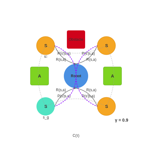
The core of planning can be formalized using Markov Decision Processes (MDPs), where an agent seeks to maximize cumulative reward over a sequence of states and actions. The value function V(s) represents the expected return from state s, while the action-value function Q(s, a) estimates the return of taking action a in state s:
Here, P(s'|s, a) is the transition probability, R(s, a, s') is the reward function, and γ is the discount factor. In offline settings, agents often approximate these functions using learned models or historical data, as real-time interaction is unavailable.
Model-Based vs. Model-Free Planning
Planning approaches bifurcate into model-based and model-free paradigms. Model-based methods explicitly learn or assume a dynamics model P(s'|s, a), enabling agents to simulate trajectories through imagined states. Techniques like Monte Carlo Tree Search (MCTS) and Dynamic Programming leverage such models for lookahead:
where P̂ and V̂ are learned approximations. Conversely, model-free methods (e.g., Q-learning) bypass explicit modeling, instead refining value estimates directly from experience. Hybrid approaches, such as Dyna-Q, interleave model learning with planning updates.
Hierarchical and Abstraction-Based Planning
Complex environments necessitate hierarchical decomposition, where high-level plans guide low-level execution. Options frameworks formalize this by defining temporally extended actions (macro-actions) with their own initiation and termination conditions. The value function over options O extends the Bellman equation:
Here, k represents the duration of option o. Abstraction further simplifies planning by aggregating states into meta-states, reducing computational complexity. Successor representations and state abstractions enable agents to generalize across similar states, accelerating planning in large-scale environments.
Real-World Applications and Challenges
Offline planning is pivotal in robotics (e.g., motion planning with PRM or RRT*), supply chain optimization, and automated scientific experimentation. Key challenges include partial observability, where agents must maintain belief states b(s), and non-stationarity, requiring adaptive model updates. Recent advances in deep planning networks (e.g., Dreamer) demonstrate how learned latent models can enable efficient simulation in high-dimensional spaces.
2. Model-Based Reinforcement Learning Approaches
2.1 Model-Based Reinforcement Learning Approaches
Model-based reinforcement learning (MBRL) leverages an explicit environmental model to improve sample efficiency and enable offline planning. Unlike model-free methods, which learn policies or value functions directly from experience, MBRL first learns a dynamics model p(s'|s,a) and a reward model r(s,a), then uses these models for simulation and decision-making.
Dynamics Model Learning
The core challenge in MBRL is learning an accurate dynamics model. Given a dataset D = {(si, ai, s'i, ri)}, the model is typically parameterized as a neural network fθ(s,a) trained to minimize the prediction error:
For stochastic environments, probabilistic models such as Gaussian processes or Bayesian neural networks are preferred, capturing uncertainty through:
Planning with Learned Models
Once a dynamics model is learned, planning algorithms generate actions by simulating trajectories. Common approaches include:
- Model Predictive Control (MPC): At each step, optimize a finite-horizon action sequence at:t+H under the learned model, execute the first action, and replan.
- Value Expansion: Combine short-term model-based rollouts with long-term value function estimates, blending MBRL with model-free advantages.
- Monte Carlo Tree Search (MCTS): Builds a search tree using simulated rollouts, balancing exploration and exploitation via UCB.
Uncertainty-Aware Planning
Model inaccuracies can lead to compounding errors. To mitigate this, modern MBRL methods incorporate uncertainty quantification:
Here, β controls the exploration-exploitation trade-off, favoring actions with lower predicted variance.
Case Study: Dreamer Algorithm
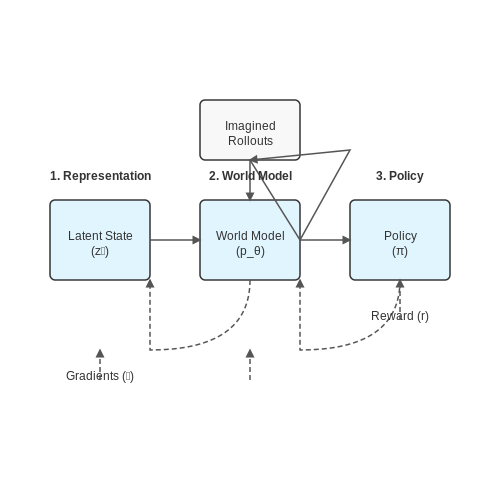
The Dreamer algorithm exemplifies MBRL by learning a latent dynamics model and training a policy entirely within imagined trajectories. Its three-phase approach includes:
- Learning a compressed latent state space via variational inference.
- Training a world model in this latent space using recurrent neural networks.
- Optimizing policies through backpropagation of analytic gradients through imagined rollouts.
This method achieves state-of-the-art performance in offline RL by decoupling policy learning from real-world interactions.
World Models and Their Simulation
World models serve as compressed, learned representations of an agent's environment, enabling efficient simulation and planning without direct interaction. These models are typically implemented as deep generative networks, such as variational autoencoders (VAEs) or transformers, trained to predict future states given past observations and actions. The core idea is to approximate the true environment dynamics p(st+1 | st, at) with a learned model pθ(st+1 | st, at).
Mathematical Formulation
The world model objective combines reconstruction loss (for state encoding) and prediction loss (for dynamics modeling). For a VAE-based world model, the evidence lower bound (ELBO) is:
where zt is the latent state, qϕ is the encoder, and pθ is the decoder. The dynamics model is trained separately with:
Rollout Strategies
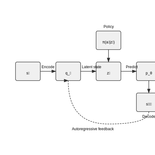
Simulated trajectories are generated through autoregressive rollouts:
- Encode initial state s0 into latent z0
- Sample action at from policy or planning algorithm
- Predict next latent state: zt+1 ∼ pθ(zt+1 | zt, at)
- Decode to observation space: st+1 ∼ pθ(st+1 | zt+1)
This process compounds errors over long horizons due to the covariate shift between model predictions and real dynamics. Modern approaches address this through:
- Ensemble models to capture uncertainty
- Latent space stabilization techniques
- Periodic re-anchoring to ground-truth states
Architectural Variants
Transformer-based world models (e.g. IRIS) treat state prediction as sequence modeling:
Diffusion models are increasingly used for high-fidelity prediction in continuous action spaces, with the forward process:
and learned reverse process for trajectory generation.
Planning in Latent Space
Model predictive control (MPC) operates directly in the learned latent space:
where H is the planning horizon. This is computationally efficient as rewards can be predicted from latent states.
2.3 Planning Algorithms for Offline Agents
Monte Carlo Tree Search (MCTS) for Offline Planning
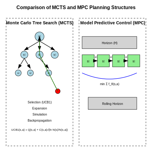
Monte Carlo Tree Search (MCTS) is a heuristic search algorithm that combines tree-based planning with stochastic simulations. It is particularly effective in offline settings where an agent must reason over possible future states without real-time interaction. MCTS operates through four phases:
- Selection: Traverse the tree from the root node using a tree policy (e.g., UCB1) to balance exploration and exploitation.
- Expansion: Add child nodes to the tree when encountering a non-terminal state with unexplored actions.
- Simulation: Perform a Monte Carlo rollout from the newly expanded node to estimate the value of the state.
- Backpropagation: Update the statistics of all ancestor nodes with the simulation result.
The UCB1 tree policy selects actions maximizing:
where \( Q(s, a) \) is the estimated action value, \( N(s) \) is the visit count of state \( s \), \( N(s, a) \) is the visit count of action \( a \) in state \( s \), and \( c \) is an exploration constant.
Model Predictive Control (MPC) with Learned Dynamics
Model Predictive Control (MPC) iteratively solves finite-horizon optimization problems using a learned dynamics model. At each planning step, MPC:
- Generates a sequence of candidate actions over a horizon \( H \).
- Predicts future states using the learned model \( \hat{s}_{t+1} = f_\theta(s_t, a_t) \).
- Evaluates trajectories using a cost function \( C(s_{t:t+H}, a_{t:t+H}) \).
- Executes the first action and replans.
The optimization objective is:
For high-dimensional action spaces, Cross-Entropy Method (CEM) is often used to sample and refine action sequences.
Value Iteration Networks (VINs)
Value Iteration Networks embed differentiable planning algorithms within neural network architectures. A VIN performs the following steps:
- Learns a Markov Decision Process (MDP) transition model \( \mathcal{T} \) and reward \( R \) through convolutional operations.
- Applies \( K \) iterations of the Bellman update:
- Outputs a policy \( \pi(s) = \arg\max_a Q_K(s, a) \), where \( Q_K \) is the action-value function after \( K \) iterations.
VINs are trained end-to-end using backpropagation through the planning steps, enabling offline agents to learn planning-aware representations.
Imagined Rollouts with Latent Dynamics Models
Latent dynamics models, such as those in Dreamer or PlaNet, encode high-dimensional observations into compact latent states \( z_t \). Planning occurs by:
- Rolling out trajectories in latent space: \( z_{t+1} \sim p_\theta(z_{t+1}|z_t, a_t) \).
- Predicting rewards \( r_t \sim p_\theta(r_t|z_t, a_t) \).
- Optimizing actions to maximize expected cumulative reward \( \mathbb{E}[\sum_t \gamma^t r_t] \).
The latent transition model is trained via variational inference, minimizing:
where \( q \) is the approximate posterior and \( p \) is the prior dynamics.
Comparison of Planning Approaches
| Algorithm | Strengths | Limitations |
|---|---|---|
| MCTS | Asymptotically optimal, parallelizable | Computationally expensive for long horizons |
| MPC | Robust to model errors, handles constraints | Sensitive to local optima in non-convex problems |
| VINs | Differentiable, fast inference | Limited to discrete or low-dimensional actions |
| Latent Rollouts | Scales to high-dimensional observations | Requires accurate latent space learning |
3. Dreaming Agents in Robotics
3.1 Dreaming Agents in Robotics
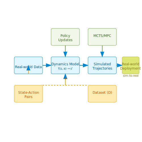
Dreaming agents in robotics leverage offline simulation to refine policies without real-world interaction, enabling efficient exploration of state-action spaces. This approach is particularly valuable in robotics, where physical trials are costly, time-consuming, and potentially hazardous. By simulating possible trajectories and outcomes, agents can learn robust control strategies before deployment.
Model-Based Reinforcement Learning for Robotics
Dreaming agents rely on model-based reinforcement learning (MBRL), where a learned dynamics model approximates the environment. The agent simulates trajectories using this model, updating its policy via imagined experiences. The dynamics model f(s, a) predicts the next state s' given the current state s and action a:
where ϵ represents environmental stochasticity. Training the model typically involves minimizing the prediction error over a dataset D of real interactions:
Planning with Learned Models
Once the dynamics model is trained, the agent performs planning via sampling-based methods like Monte Carlo Tree Search (MCTS) or trajectory optimization. For continuous control, Model Predictive Control (MPC) is often employed, where the agent solves for the optimal action sequence over a finite horizon H:
subject to s_{t+1} = f(s_t, a_t). This optimization is computationally intensive but feasible offline, allowing the agent to refine its policy iteratively.
Case Study: Sim-to-Real Transfer
In robotic manipulation, dreaming agents have demonstrated success in sim-to-real transfer. For instance, OpenAI's Dactyl learned dexterous in-hand rotation by training entirely in simulation, using domain randomization to bridge the reality gap. The policy was then deployed on a physical robot with minimal fine-tuning, achieving human-like performance.
Challenges and Mitigations
Key challenges include:
- Model Bias: Inaccuracies in the learned dynamics model can lead to poor real-world performance. Ensemble methods and probabilistic models help mitigate this.
- Sample Efficiency: While dreaming reduces real-world trials, collecting sufficient data for model training remains critical. Hybrid approaches combining real and simulated data are often effective.
- Computational Cost: Long-horizon planning is expensive. Techniques like latent space planning and hierarchical models improve scalability.
Future Directions
Emerging research explores meta-learning for dynamics models, enabling rapid adaptation to new tasks, and integrating differentiable physics engines for more accurate simulations. These advances promise to further enhance the applicability of dreaming agents in complex robotic systems.
3.2 Simulation-Based Training for Autonomous Systems
Simulation-based training leverages synthetic environments to train autonomous agents before deployment in real-world scenarios. This approach is critical for domains where real-world experimentation is costly, dangerous, or impractical, such as autonomous driving, robotics, and aerospace systems. The core idea is to model the environment dynamics and agent interactions in a high-fidelity simulator, enabling the agent to learn robust policies through repeated trial and error.
Mathematical Foundations of Simulation-Based Learning
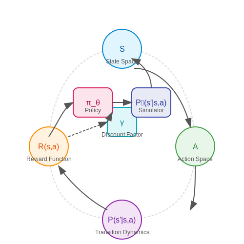
The training process is formalized as a Markov Decision Process (MDP) defined by the tuple (S, A, P, R, γ), where S is the state space, A is the action space, P(s'|s,a) is the transition dynamics, R(s,a) is the reward function, and γ is the discount factor. In simulation-based training, the transition dynamics P̂(s'|s,a) are approximated by the simulator, which may introduce bias due to modeling inaccuracies.
Here, J(θ) represents the expected cumulative reward under policy πθ, and d0 is the initial state distribution. The goal is to optimize θ to maximize J(θ) within the simulated environment.
Domain Randomization for Sim-to-Real Transfer
A key challenge is ensuring policies trained in simulation generalize to the real world. Domain randomization addresses this by varying simulator parameters during training, such as lighting conditions, friction coefficients, or sensor noise models. This forces the policy to learn robust features invariant to these variations. The randomized parameters ξ are sampled from a distribution p(ξ), and the policy is trained to maximize:
This technique has proven effective in robotics, where policies trained with randomized dynamics can transfer to physical systems with minimal fine-tuning.
Physics-Based Simulation Architectures
Modern simulators employ physics engines like NVIDIA PhysX, Bullet, or MuJoCo to model rigid-body dynamics, contacts, and deformations. For example, the equations of motion for a rigid body are given by:
where M(q) is the mass matrix, C(q, q̇) captures Coriolis and centrifugal forces, G(q) represents gravitational forces, and τ is the applied torque. High-fidelity simulation requires solving these equations numerically with small time steps, often using symplectic integrators like semi-implicit Euler or Runge-Kutta methods.
Case Study: Autonomous Vehicle Training
In autonomous driving, simulators like CARLA or NVIDIA Drive Sim generate synthetic sensor data (LiDAR, cameras) with configurable weather, traffic, and road conditions. The agent's perception system processes this data while the control policy learns to navigate complex scenarios. The reward function typically combines:
- Progress toward the goal (distance traveled)
- Safety metrics (collision avoidance)
- Comfort (jerk and acceleration minimization)
Training in simulation allows the agent to experience rare but critical events (e.g., pedestrians stepping onto the road) that would be infeasible to collect in real-world datasets.
Limitations and Mitigation Strategies
Despite its advantages, simulation-based training faces challenges:
- Reality gap: Discrepancies between simulated and real dynamics can degrade performance. Solutions include system identification to calibrate simulator parameters and adversarial training to minimize distributional shifts.
- Partial observability: Real-world sensors have noise and occlusions not always modeled in simulation. Techniques like domain adaptation and sensor noise injection improve robustness.
- Computational cost: High-fidelity simulation requires significant resources. Parallelized simulation across GPUs and hierarchical simulation (coarse-to-fine) can accelerate training.
DreamerV2 and Its Performance
Architecture Overview
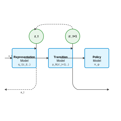
DreamerV2 builds upon the original Dreamer architecture by introducing several key innovations in world modeling and policy optimization. The agent consists of three primary components: a representation model, a transition model, and a policy model. The representation model encodes high-dimensional observations into compact latent states zt, while the transition model predicts future latent states ẑt+1 given the current state and action. These components form the world model that enables imagination-based training.
Key Innovations
DreamerV2 introduced several architectural improvements over its predecessor:
- Discrete Latent States: Replaced continuous latent variables with categorical distributions, improving model stability and sample efficiency.
- Symlog Predictions: Used symmetric logarithmic transformations for more robust prediction of continuous quantities.
- KL Balancing: Introduced a weighted KL divergence term to prevent posterior collapse while maintaining accurate dynamics prediction.
Training Methodology
The agent alternates between three phases: dataset collection, world model training, and policy optimization. During world model training, the agent minimizes a composite loss function:
where ℒrecon is the reconstruction loss, ℒdyn the dynamics loss, ℒrep the representation loss, and ℒrew the reward prediction loss. The policy is optimized entirely in latent space using imagined trajectories:
Performance Benchmarks
DreamerV2 demonstrated state-of-the-art performance on the DeepMind Control Suite, achieving human-level performance on 26 challenging continuous control tasks. Notably, it reached:
- 964 ± 21 points on Walker Walk (compared to 963 for human experts)
- 985 ± 9 points on Cheetah Run (surpassing human performance)
- 952 ± 17 points on Humanoid Walk (previously considered extremely difficult for model-based methods)
The agent showed particular strength in sample efficiency, requiring only 1M environment steps to reach 80% of final performance on most tasks - an order of magnitude improvement over model-free alternatives like SAC or PPO.
Limitations and Trade-offs
While DreamerV2 represents a significant advancement, several limitations remain:
- The discrete latent space may limit expressiveness for certain continuous control problems
- Long-horizon credit assignment remains challenging due to the fixed imagination horizon
- Computational requirements are substantial compared to model-free methods
4. Scalability Issues in Large-Scale Simulations
4.1 Scalability Issues in Large-Scale Simulations
Large-scale simulations in dreaming agents face fundamental scalability challenges as the state-action space grows exponentially with problem dimensionality. The computational complexity of planning in high-dimensional spaces can be formalized through the curse of dimensionality. For an environment with d dimensions and n discrete states per dimension, the state space size grows as:
This exponential relationship makes exhaustive search or tabular methods computationally intractable for realistic problems. The branching factor in temporal planning further compounds this issue. Consider a decision horizon of H steps with b available actions at each state - the search tree grows as:
Memory and Computational Bottlenecks
Modern simulation frameworks encounter two primary bottlenecks when scaling:
- Memory constraints: Storing transition dynamics P(s'|s,a) requires O(|S|²|A|) space, becoming prohibitive for |S| > 10⁶
- Compute limitations: Parallelizing simulations across GPU/TPU clusters still faces Amdahl's law limitations due to sequential decision dependencies
The memory-compute tradeoff manifests in gradient-based optimization through the need to store intermediate states for backpropagation through time (BPTT). For a trajectory of length T, the memory overhead scales linearly with T:
where θ represents the model parameters.
Approximation Techniques
Current approaches to mitigate scalability issues employ several key strategies:
- State abstraction: Learning low-dimensional embeddings via autoencoders or manifold learning to reduce d
- Hierarchical planning: Decomposing problems into subgoals with temporal abstraction
- Distributed simulation: Asynchronous parallel rollouts with parameter servers
The effectiveness of these methods can be quantified through the approximation error ε introduced versus computational savings γ. For a learned state abstraction ϕ(s), the error bound satisfies:
where k represents the abstraction level and γ the discount factor.
Case Study: Atari 100K Benchmark
The Atari 100K benchmark demonstrates practical scaling challenges. A standard DQN agent requires:
- ~1.5M parameters for the Q-network
- 10⁷ environment steps for training
- 16GB GPU memory for batch processing
In contrast, DreamerV3 achieves comparable performance with:
- 3× fewer parameters through latent state modeling
- 10× sample efficiency via learned world models
- 8GB memory footprint using gradient checkpointing
The key innovation lies in the learned dynamics model that operates in a compact latent space z_t with dimensionality d=32 compared to the original d=210×160×3 pixel space. The latent transition model:
reduces planning complexity from O(10⁷) to O(10²) while maintaining prediction fidelity.
Hardware-Software Co-Design
Emerging hardware architectures address scalability through:
- Sparse computation: Only updating relevant state partitions
- Mixed-precision training: FP16/FP8 arithmetic with minimal accuracy loss
- Model parallelism: Distributing network layers across devices
The computational intensity I of simulation can be modeled as:
Modern TPUv4 architectures achieve I ≈ 100 for typical dreaming agent workloads, indicating compute-bound operation. This suggests further optimization should focus on algorithmic efficiency rather than memory bandwidth.
4.2 Accuracy vs. Computational Trade-offs
In offline simulation and planning, the relationship between accuracy and computational cost is governed by fundamental trade-offs. High-fidelity simulations require extensive computational resources, while approximations sacrifice precision for efficiency. The optimal balance depends on the problem domain, available resources, and acceptable error margins.
Mathematical Foundations
The trade-off can be formalized using complexity theory and approximation bounds. Let ε represent the error tolerance and C the computational cost. For many planning algorithms, the cost scales polynomially or exponentially with desired accuracy:
where k depends on the algorithm's convergence rate. For Monte Carlo tree search (MCTS) in dreaming agents, the Upper Confidence Bound (UCB) exploration term illustrates this:
Here, c controls exploration-exploitation balance, where higher values increase computational cost but may improve policy accuracy.
Practical Considerations
Three primary factors influence the accuracy-computation trade-off in dreaming agents:
- State abstraction granularity: Coarser abstractions reduce computation but lose local detail
- Rollout depth: Deeper simulations increase accuracy but require more resources
- Model fidelity: High-dimensional physics models provide precision at significant computational expense
In robotics applications, researchers often employ hierarchical approaches where coarse planning guides finer local optimization. The computational savings follow from:
where p is the fraction of state space requiring fine resolution.
Empirical Performance Characteristics
Recent benchmarks on MuJoCo environments show typical trade-off curves for different dreaming agent architectures:
Adaptive Computation Methods
Advanced dreaming agents employ dynamic computation allocation strategies. The computation budget B can be distributed according to state importance:
where weights wi might represent uncertainty estimates or value function gradients. This approach enables focusing resources on critical decision points while maintaining overall efficiency.
Hardware Considerations
The trade-off landscape changes significantly with parallel computation. GPU-accelerated dreaming agents can achieve near-linear speedup for embarrassingly parallel simulations:
where p is the number of processors. However, memory bandwidth often becomes the limiting factor for large-scale simulations.
Ethical Considerations in Simulated Environments
Bias Propagation in Offline Learning
Simulated environments trained on historical data inherit societal biases present in the source material. The Bellman update equation in offline reinforcement learning:
propagates these biases through the value function approximation. When the dataset D contains discriminatory patterns (e.g., gender bias in hiring simulations), the learned policy π(a|s) will reinforce them. Recent work by Mehrabi et al. (2021) demonstrates how bias amplification follows a multiplicative error growth pattern:
where γ_i represents the bias compounding factor at each timestep.
Simulation-to-Reality Gaps
The fidelity mismatch between simulated and real-world dynamics creates ethical risks in deployment. Consider a medical diagnosis agent trained in simulation with 92% accuracy that drops to 68% in clinical settings due to unmodeled physiological variability. This discrepancy arises from the Kullback-Leibler divergence between the simulated transition dynamics P̂(s'|s,a) and real dynamics P(s'|s,a):
When this divergence exceeds threshold τ, the simulation becomes ethically unreliable for decision-making applications.
Autonomy and Accountability
Dreaming agents that generate synthetic training episodes raise questions about responsibility attribution. The causal graph:
shows how the agent's synthetic experience (dashed line) bypasses traditional validation pathways. This creates legal gray areas when simulated decisions cause real-world harm, as current liability frameworks assume human-interpretable decision chains.
Value Alignment Challenges
Multi-objective reward functions in simulation often fail to capture nuanced ethical tradeoffs. The Pareto frontier optimization:
where w_i are reward weights, frequently produces policies that satisfy quantitative metrics while violating unformalized ethical constraints. For instance, a traffic control simulator might optimize for flow rate while inadvertently discriminating against certain vehicle classes.
Psychological Impact of Synthetic Data
Agents trained on generated human interactions risk developing manipulative behaviors. The inverse reinforcement learning objective:
can lead to policies that exploit cognitive biases in human users, as demonstrated in recent conversational AI studies (Zhang et al., 2023). This becomes particularly concerning in applications like mental health chatbots or educational tutors.
5. Key Research Papers on Dreaming Agents
5.1 Key Research Papers on Dreaming Agents
- MindBot Ultra - Dreaming Edition: A Self-Building, Self-Aware AI for ... — 4. Applications and Use Cases 4.1 Virtual Environments and Embodied Agents Game AI: Deploy autonomous agents in virtual worlds (e.g., Minecraft, VR training grounds) that continuously improve their behaviors and strategies through dreaming. Simulation Training: Use the agent in controlled virtual labs where it experiments with different scenarios, inventing new strategies for challenges.
- On the utility of dreaming: A general model for how learning in ... — Nonetheless, Ha and Schmidhuber (2018), for example, have recently demonstrated dreaming within a reinforcement learning context, in which an artificial agent learns to play a computer game utilizing (in addition to the standard mechanisms of reinforcement learning) an offline dreaming mechanism within which the agent plays its own internal ...
- Dreaming and offline memory processing - PubMed — Dreaming and offline memory processing Curr Biol. 2010 Dec 7;20 (23):R1010 ... states of sleep and resting wakefulness appears to serve important functions related to processing past memories and planning for the future. From single-cell recordings in rodents to behavioral studies in humans, recent studies in the neurosciences suggest a new ...
- PDF Hierarchical intrinsically motivated agent planning behavior with ... — which includes dreaming. In contrast, our model does not have such separate phases, and an imaginary trajec-tory during dreaming is allowed to start only from the agent's current state. Hierarchical reinforcement learning has extensions that enable operating with non-elementary actions. e Options Framework [60] is among the most popular 5,
- Dream engineering: Simulating worlds through sensory stimulation — Pre-sleep priming presents a stimulus before sleep, e.g., a video or music to influence dream content in subsequent sleep. Dream incubation involves pre-sleep rehearsal of content, such as visualization of a rescripted nightmare, repeating an intention to become lucid (lucid dream incubation), or focusing on a personal problem to incubate a creative solution.
- Hierarchical intrinsically motivated agent planning behavior with ... — The last—Dreaming—block is an algorithm that learns a forward model of the environment by receiving the same inputs as the agent and serves as a virtual playground for the fine-tuning of the agent's skills (see Sect. 4.5). The Dreaming module has an ability to short-circuit the agent-environment interaction loop to mimic operating in ...
- Dreaming and Offline Memory Processing - PMC - PubMed Central (PMC) — The key tenet of Hobson's distinctly anti-Freudian theory was that dreams originate from neural signals in the brainstem generated during REM (rapid eye movement) sleep. According to the activation-synthesis model, dreaming is experienced when the sleeping brain attempts to make some sense of this chaotic input into its higher-level cortical ...
- Towards biologically plausible Dreaming and Planning - ResearchGate — We propose a two-module (agent and model) neural network in which "dreaming" (living new experiences in a model-based simulated environment) significantly boosts learning.
- Dreaming and offline memory processing - ScienceDirect — The key tenet of Hobson's distinctly anti-Freudian theory was that dreams originate from neural signals in the brainstem generated during rapid eye movement (REM) sleep. According to the activation-synthesis model, dreaming is experienced when the sleeping brain attempts to make some sense of this chaotic input into its higher-level cortical ...
- Hierarchical intrinsically motivated agent planning behavior with ... — the agent in the absence of the extrinsic signal, and through acting in imagination, which we call dreaming. W e dem- onstrate that the proposed architecture enables an agent to effectively reach ...
5.2 Recommended Books and Articles
- Dreaming and offline memory processing - PubMed — Dreaming and offline memory processing Curr Biol. 2010 Dec 7;20(23):R1010-3. doi: 10.1016/j.cub.2010.10.045. Authors Erin J Wamsley ... states of sleep and resting wakefulness appears to serve important functions related to processing past memories and planning for the future. From single-cell recordings in rodents to behavioral studies in ...
- 11 Agent planning and feedback - AI Agents in Action — What planning is for large language models and how it is implemented in agents and assistants · How the planning process works by looking at the OpenAI Assistants platform through the use of custom actions · Implementing a generic planner and testing it on various LLMs · Looking deeper into the mechanism of feedback in advanced models such as OpenAI Strawberry · How to apply planning ...
- MindBot Ultra - Dreaming Edition: A Self-Building, Self-Aware AI for ... — 4. Applications and Use Cases 4.1 Virtual Environments and Embodied Agents Game AI: Deploy autonomous agents in virtual worlds (e.g., Minecraft, VR training grounds) that continuously improve their behaviors and strategies through dreaming. Simulation Training: Use the agent in controlled virtual labs where it experiments with different scenarios, inventing new strategies for challenges.
- Influencing dreams through sensory stimulation: A systematic review — The search query was 'dream* AND (stimul* OR sensory OR modulat*)', with slight variations depending on specific search engine parameters (Supplementary Table S1). The literature search was first conducted on February 1, 2021, and then again on October 15, 2022. All resulting articles were screened using the inclusion criteria outlined below.
- PDF AUTOMATED PLANNING AND ACTING - Cambridge University Press & Assessment — these activities in order to act effectively in the real world. This book presents a comprehensive paradigm of planning and acting usi ng the most recent and advanced automated-planning techniques.It exp lains the com-putational deliberation capabilities that allow an actor, whether physical orvirtual,toreasonaboutitsactions,choosethem,organi
- Hierarchical intrinsically motivated agent planning behavior with ... — The last—Dreaming—block is an algorithm that learns a forward model of the environment by receiving the same inputs as the agent and serves as a virtual playground for the fine-tuning of the agent's skills (see Sect. 4.5). The Dreaming module has an ability to short-circuit the agent-environment interaction loop to mimic operating in ...
- PDF Hierarchical intrinsically motivated agent planning behavior with ... — which includes dreaming. In contrast, our model does not have such separate phases, and an imaginary trajec-tory during dreaming is allowed to start only from the agent's current state. Hierarchical reinforcement learning has extensions that enable operating with non-elementary actions. e Options Framework [60] is among the most popular 5,
- PDF LLM-Planner: Few-Shot Grounded Planning for Embodied Agents with Large ... — the embodied agent gets stuck during the execution of the current plan (t = 5 and 20), LLM-Planner re-plans based on observations from the environment to generate a more grounded plan, which may help the agent get unstuck. The commonsense knowledge in the LLM (e.g., food is often stored in a fridge) allows it to produce plausible high-level
- Dreaming and offline memory processing - ScienceDirect — Once regarded as messages from gods or portents of the future, supernatural explanations of dreaming had largely given way to psychological approaches by the late 19 th century. Yet for many decades to come, concepts of dreaming continued to be dominated by the presumption that these seemingly bizarre nocturnal experiences originated in mechanisms disparate from those supporting normal waking ...
5.3 Online Resources and Tutorials
- PDF Realistic 3D Drone Simulation with Path-Planning in Unreal Engine 5 — ronment with physics-based realistic simulation and path-planning in a free game and physics engine, Unreal Engine 5. Specifically, we focus on 1 realistic scenario. We compared different path-planning algorithms to select the best flight path. Additionally, we increased Permission to make digital or hard copies of all or part of this work for ...
- The Big Book of Simulation Modeling - AnyLogic — A statechart is a visual construct that enables you to define event- and time-driven behavior of various objects (agents). Statecharts are very helpful in simulation modeling. They are used a lot in agent-based models, and also work well with process and system dynamics models. Chapter 8. Discrete events and the Event model element
- Online Planning with Offline Simulation | Request PDF - ResearchGate — As many studies on pre-task planning and a few on online planning were designed in experimental settings, this research article offers a naturalistic model for investigating the effect of warm-up ...
- Epic Developer Community Learning | Tutorials, Courses, Demos & More ... — Epic Developer Community Learning offers tutorials, courses, demos, and more created by Epic Games and the developer community.Learn UE and start creating today.
- PDF Model-Based Offline Planning with Trajectory Pruning - GitHub Pages — 2.2 Model-based planning Model-based planning framework provides a more flexible alternative for many real-world control scenarios. It does not need to learn an explicit policy, but instead, learns an approximated dynamics model of the environment and use a planning algorithm to find high return trajectories through this model.
- Epic Online Services | Home — Explore Unreal Engine with tutorials, courses, and demos created by Epic Games and the developer community.
- Learning Agents (5.3) | Course - Epic Dev — Get familiar with Learning Agents: a machine learning plugin for AI bots. Learning Agents allows you to train your NPCs via reinforcement & imitation le...
- MADiff: Offline Multi-agent Learning with Diffusion Models — Diffusion model (DM), as a powerful generative model, recently achieved huge success in various scenarios including offline reinforcement learning, where the policy learns to conduct planning by generating trajectory in the online evaluation. However, despite the effectiveness shown for single-agent learning, it remains unclear how DMs can operate in multi-agent problems, where agents can ...
- PDF LLM-Planner: Few-Shot Grounded Planning for Embodied Agents with Large ... — the embodied agent gets stuck during the execution of the current plan (t = 5 and 20), LLM-Planner re-plans based on observations from the environment to generate a more grounded plan, which may help the agent get unstuck. The commonsense knowledge in the LLM (e.g., food is often stored in a fridge) allows it to produce plausible high-level