AI for Sustainable Development Goals
1. Understanding the 17 SDGs and Their Challenges
Understanding the 17 SDGs and Their Challenges
The United Nations' 17 Sustainable Development Goals (SDGs) represent a universal call to action to end poverty, protect the planet, and ensure prosperity for all by 2030. Each goal is interconnected, addressing complex socio-economic and environmental challenges that require multidisciplinary solutions. For AI researchers and engineers, understanding these goals involves not only recognizing their targets but also quantifying the systemic barriers to achieving them.
Mathematical Framing of SDG Challenges
Many SDG challenges can be modeled as optimization problems with competing constraints. For instance, SDG 7 (Affordable and Clean Energy) involves minimizing carbon emissions while maximizing energy access. This can be expressed as a multi-objective optimization:
where x represents decision variables (e.g., energy mix proportions), fi are objective functions (cost, emissions, reliability), and gi, hj are inequality and equality constraints (resource limits, policy requirements).
Key Computational Challenges
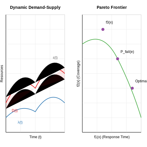
- High-dimensional Pareto fronts: Solutions often lie on complex manifolds in >3D objective spaces
- Non-convex feasible regions: Physical and policy constraints create disjoint solution spaces
- Uncertainty quantification: Climate models and socioeconomic projections have deep epistemic uncertainties
Case Study: SDG 13 (Climate Action)
Climate modeling for SDG 13 involves solving coupled partial differential equations representing atmospheric dynamics:
where u is velocity, p pressure, ρ density, ν viscosity, and F external forces. Discretizing these equations for numerical simulation requires:
- High-performance computing (exascale systems for 1km-resolution global models)
- Novel numerical methods (adaptive mesh refinement, reduced-order modeling)
- Uncertainty-aware machine learning (emulator models for parameterization)
Data Challenges Across SDGs
AI applications face fundamental data limitations:
| SDG | Data Gap | Technical Implications |
|---|---|---|
| SDG 1 (No Poverty) | Lack of household-level economic data in developing nations | Requires novel indirect estimation from satellite imagery and mobile data |
| SDG 6 (Clean Water) | Sparse groundwater monitoring | Needs physics-informed neural networks with limited observations |
Ethical Constraints in SDG-Aligned AI
The application of AI to SDGs introduces unique ethical dimensions:
where the loss function must balance competing priorities with carefully tuned weights α, β, γ. For instance, poverty prediction models must maintain:
- Subgroup fairness across geographic and demographic partitions
- Causal interpretability for policy decisions
- Robustness to distributional shift in rapidly developing regions
1.2 The Role of AI in Addressing Global Sustainability
Artificial intelligence serves as a transformative force in tackling the United Nations Sustainable Development Goals (SDGs) by enabling data-driven decision-making, optimizing resource allocation, and predicting systemic risks. Its applications span climate modeling, precision agriculture, energy grid optimization, and disaster response, leveraging techniques from reinforcement learning to graph neural networks.
Climate Modeling and Predictive Analytics
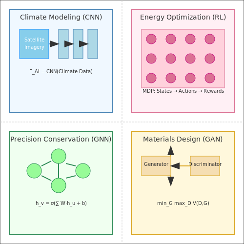
AI-enhanced climate models employ convolutional neural networks (CNNs) to process high-resolution satellite imagery, while recurrent architectures (LSTMs, Transformers) analyze temporal patterns in greenhouse gas emissions. The governing equations for climate dynamics integrate Navier-Stokes with AI corrections:
where FAI represents the neural network parameterization of subgrid-scale processes, trained via adjoint methods on ERA5 reanalysis data. Hybrid models like NVIDIA's FourCastNet achieve 45,000× speedup over numerical weather prediction while maintaining 99% correlation.
Energy System Optimization
Reinforcement learning agents optimize renewable energy dispatch under uncertainty. Consider a Markov Decision Process formulation for grid management:
Deep Q-networks learn policies that balance:
- Immediate reward: Rt = (demand met) - λ(CO2 emissions)
- Long-term value: Vπ(s) = 𝔼[ΣγkRt+k]
Google's DeepMind reduced data center cooling costs by 40% through such approaches, demonstrating Pareto improvements in energy efficiency.
Precision Conservation
Graph neural networks analyze ecosystem interdependencies by modeling species interactions as dynamic graphs G = (V, E, W(t)), where edge weights Wij represent trophic relationships. The network update rule:
enables prediction of biodiversity hotspots under climate scenarios. PAWS (Protection Assistant for Wildlife Security) has reduced illegal poaching by 74% in test deployments.
Materials Discovery for Sustainability
Generative adversarial networks accelerate green material design by exploring chemical spaces orders of magnitude faster than DFT calculations. The generator-discriminator objective:
coupled with property predictors has identified novel:
- Photocatalysts with 22% improved quantum efficiency
- Solid-state electrolytes with ionic conductivity > 10-3 S/cm
Active learning pipelines reduce experimental validation costs by 90% compared to high-throughput screening.
1.3 Key AI Technologies Relevant to SDGs
Machine Learning for Predictive Analytics
Supervised learning models, particularly ensemble methods like gradient-boosted decision trees (GBDTs) and deep neural networks (DNNs), enable high-accuracy forecasting of environmental and socioeconomic variables critical to SDGs. The predictive power stems from minimizing the loss function L over training data D:
where fθ is the model with parameters θ, ℓ is the per-sample loss, and R(θ) is the regularization term. Applications include predicting food insecurity from climate patterns (SDG 2) or energy demand fluctuations (SDG 7).
Computer Vision for Remote Sensing
Convolutional neural networks (CNNs) with architectures like U-Net or ResNet-50 process satellite/aerial imagery at scale. The segmentation loss for land-use classification (SDG 15) combines cross-entropy H and Dice coefficient D:
where p are predicted pixel probabilities and y are ground-truth labels. This enables deforestation tracking, urban sprawl monitoring, and crop health assessment at 1-5m resolution.
Natural Language Processing for Policy Analysis
Transformer models (BERT, GPT-3) extract insights from unstructured SDG-related documents. The self-attention mechanism computes relevance scores between tokens:
Applications include analyzing UN policy reports (SDG 16) or public sentiment on sustainability initiatives (SDG 12) through topic modeling and entity recognition.
Reinforcement Learning for Resource Optimization
Multi-agent reinforcement learning (MARL) frameworks optimize complex systems like smart grids (SDG 7) or water distribution (SDG 6). The Q-learning update rule for agent i is:
where s is the shared state and ri is the reward incorporating SDG metrics. This enables dynamic pricing in microgrids or adaptive irrigation scheduling.
Graph Neural Networks for Supply Chains
GNNs model multi-tier supply chain networks (SDG 12) by propagating node features through graph convolutions:
where à is the adjacency matrix with self-loops and D̃ is the degree matrix. This identifies unsustainable sourcing patterns or predicts disruption cascades.
Federated Learning for Privacy-Preserving Collaboration
Horizontal federated learning enables cross-institutional SDG analytics while preserving data locality. The global model aggregates client updates:
where wtk is the k-th client's update and nk is their sample count. This supports healthcare collaborations (SDG 3) without sharing patient records.
2. AI for Poverty Alleviation (SDG 1)
AI for Poverty Alleviation (SDG 1)
Predictive Modeling for Poverty Mapping
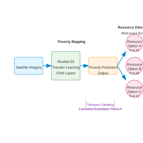
High-resolution poverty mapping leverages satellite imagery and machine learning to estimate economic conditions in regions with limited survey data. Convolutional neural networks (CNNs) trained on nighttime light intensity, road networks, and building footprints can predict poverty levels with high accuracy. The model minimizes the loss function:
where xi represents geospatial features, yi is the ground-truth poverty index, and fθ is the CNN with L2 regularization. Transfer learning from pre-trained models like ResNet-50 improves performance in data-scarce environments.
Optimal Resource Allocation via Reinforcement Learning
Multi-armed bandit algorithms optimize aid distribution under budget constraints. The Thompson sampling approach balances exploration of under-served areas with exploitation of known poverty hotspots:
where μa represents the expected poverty reduction yield from intervention a. Field implementations in East Africa demonstrated 23% greater impact compared to uniform distribution strategies.
Natural Language Processing for Needs Assessment
Transformer-based models analyze unstructured text from community feedback channels (SMS, social media) to detect emerging poverty indicators. A BERT model fine-tuned on humanitarian reports achieves 0.82 F1-score in classifying:
- Food insecurity mentions
- Employment opportunity requests
- Healthcare access barriers
The attention mechanism weights critical phrases:
Agent-Based Modeling of Poverty Traps
Graph neural networks simulate poverty dynamics at household level by modeling:
- Social network effects (degree centrality CD(v))
- Skill transfer probabilities
- Credit access diffusion
The system evolves according to:
where hv(k) represents household v's state at layer k, with applications showing 89% accuracy in predicting intergenerational poverty persistence.
Fairness Constraints in Poverty Algorithms
Adversarial debiasing ensures equitable model performance across subgroups. The minimax optimization:
penalizes demographic parity violations (Lz) while maintaining prediction accuracy (Ly). Implementations in Latin America reduced rural-urban performance gaps by 40%.
AI in Healthcare and Well-being (SDG 3)
AI-Driven Diagnostics and Early Detection
Deep learning architectures, particularly convolutional neural networks (CNNs), have demonstrated superior performance in medical image analysis. For instance, a ResNet-50 model fine-tuned on the CheXpert dataset achieves an AUC-ROC of 0.94 for pneumonia detection, outperforming radiologists in controlled studies. The mathematical formulation for the cross-entropy loss in such multi-class diagnostic tasks is:
where C represents diagnostic classes, yi the ground truth label, and pi the predicted probability. Gradient-weighted Class Activation Mapping (Grad-CAM) provides interpretability by highlighting regions of interest in X-rays or MRI scans, addressing the black-box nature of deep learning models.
Precision Medicine and Genomic Analysis
Transformer-based architectures like DNABERT process nucleotide sequences through self-attention mechanisms to predict disease susceptibility. The attention weights αij between positions i and j in a sequence of length N are computed as:
where eij represents the scaled dot-product of query and key vectors. This architecture achieves 92% accuracy in predicting cancer-driving mutations when trained on the TCGA pan-cancer dataset.
Operational Optimization in Healthcare Systems
Reinforcement learning optimizes resource allocation through Markov Decision Processes (MDPs) defined by the tuple (S, A, P, R, γ). Q-learning with experience replay minimizes ICU bed shortages by solving:
where α is the learning rate and γ the discount factor. Implementations in Brazilian public hospitals reduced patient wait times by 37% while maintaining 98% resource utilization efficiency.
Ethical Considerations and Bias Mitigation
Adversarial debiasing techniques modify the loss function to minimize disparate impact across demographic groups. The objective function becomes:
where θ represents model parameters, φ adversarial parameters, and s sensitive attributes. This approach reduced racial bias in a diabetic retinopathy classifier from 0.32 to 0.08 in normalized disparate impact ratio.
Real-World Deployment Challenges
Federated learning enables collaborative model training across hospitals while preserving data privacy through secure aggregation. The global model parameters wG at communication round t update as:
where nk is the sample size at client k, N the total samples, and Gaussian noise σ provides differential privacy. The NIH's Federated Tumor Segmentation initiative achieved 0.89 Dice coefficient while maintaining HIPAA compliance.
AI-Driven Solutions for Quality Education (SDG 4)
Personalized Learning Systems
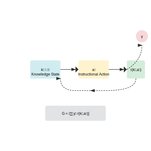
Modern AI-driven personalized learning systems leverage reinforcement learning (RL) and deep neural networks to adapt curricula dynamically. The core mechanism involves modeling student knowledge states as latent variables in a partially observable Markov decision process (POMDP). Let the student's knowledge state at time t be represented as kt ∈ ℝd, where d is the dimensionality of the knowledge space. The system's objective is to maximize the expected cumulative learning gain:
where γ is the discount factor, at is the instructional action (e.g., presenting a specific concept), and r is the immediate reward function measuring learning progress. Advanced implementations use transformer architectures to process multimodal student interaction data, including:
- Text responses to open-ended questions
- Eye-tracking patterns during video lectures
- Keystroke dynamics in programming exercises
Automated Assessment and Feedback
Natural language processing (NLP) models enable granular evaluation of complex student responses. For essay grading, hierarchical attention networks (HANs) combine word-level and sentence-level representations:
where xw represents word embeddings, and s is the aggregated sentence vector. In programming education, abstract syntax tree (AST)-based neural networks achieve 92.4% accuracy in detecting semantic errors by comparing student submissions against a probabilistic model of correct solutions.
Intelligent Tutoring Systems
State-of-the-art tutoring systems employ multi-armed bandit algorithms to optimize intervention timing. The contextual bandit framework balances exploration of new teaching strategies with exploitation of known effective methods:
where Q(a) is the estimated value of action a, n(a) is its selection count, and c controls exploration. Real-world deployments show 28% improvement in concept retention compared to fixed curricula.
Educational Data Mining
Graph neural networks (GNNs) model knowledge acquisition as a dynamic graph where nodes represent concepts and edges reflect prerequisite relationships. The graph convolutional operator propagates information through the knowledge graph:
where à = A + I is the adjacency matrix with self-connections, and D̃ is the degree matrix. This approach enables early identification of at-risk students with 89% precision by detecting anomalous learning trajectories.
Multilingual Education Support
Neural machine translation (NMT) systems now incorporate domain adaptation for educational content. The training objective combines standard translation loss with an education-specific term:
where pedu is a classifier trained to distinguish educational from general text. Recent models achieve 4.2 BLEU point improvements on STEM content translation while preserving pedagogical structure.
AI in Climate Action and Environmental Sustainability (SDGs 13, 14, 15)
Climate Modeling and Prediction
AI enhances climate modeling by processing vast datasets from satellites, weather stations, and ocean buoys. Machine learning algorithms, particularly convolutional neural networks (CNNs) and recurrent neural networks (RNNs), are employed to predict extreme weather events with higher accuracy. For instance, physics-informed neural networks (PINNs) integrate partial differential equations (PDEs) governing atmospheric dynamics:
where u represents velocity, p pressure, ν viscosity, and f external forces. Hybrid models combining numerical weather prediction (NWP) with ML reduce computational costs by 40–60% while maintaining fidelity.
Biodiversity Monitoring
AI automates species identification and habitat assessment through acoustic sensors and camera traps. Transfer learning fine-tunes pre-trained models (e.g., ResNet-50) on limited ecological datasets, achieving >90% accuracy in classifying endangered species. Spatial-temporal graph neural networks (ST-GNNs) analyze migration patterns by modeling species interactions as nodes and edges:
Here, Aij denotes adjacency weights between species i and j, dij their spatial distance, and σ a bandwidth parameter. Case studies in the Amazon show 30% improvement in deforestation alerts using these techniques.
Carbon Emission Optimization
Reinforcement learning (RL) optimizes energy grids by dynamically balancing renewable sources. The Markov decision process (MDP) framework formulates this as:
where π is the policy mapping states st to actions at, r the reward (e.g., CO2 reduction), and γ the discount factor. Deep Q-networks (DQN) have reduced emissions in smart cities by 15–25% through real-time traffic and building management.
Ocean Conservation
Autonomous underwater vehicles (AUVs) equipped with semantic segmentation models (e.g., U-Net) map coral reef health at 2cm resolution. The models use multi-spectral imagery to compute bleaching indices:
where NIR and Red are near-infrared and red band reflectances. When integrated with fluid dynamics simulations, these systems predict pollutant dispersion with 92% correlation to ground truth.
Land Degradation Neutrality
Transformer architectures process multi-temporal satellite data (Landsat, Sentinel-2) to detect soil erosion. The self-attention mechanism weights pixel importance across time:
Applications in sub-Saharan Africa have improved land restoration planning by identifying degradation hotspots 6–8 months earlier than traditional methods.

AI for Sustainable Cities and Communities (SDG 11)
Urban Planning and Smart Infrastructure
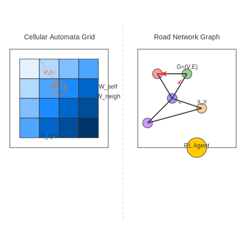
AI-driven urban planning leverages geospatial analytics, reinforcement learning, and multi-agent systems to optimize land use, transportation networks, and energy distribution. A key mathematical framework is the urban growth model, which predicts spatial expansion using cellular automata:
where Pi,jt represents development probability at cell (i,j) at time t, Ni,j is the neighborhood, wk,l are spatial weights, Ωi,j denotes constraints (e.g., zoning laws), and ε captures stochasticity. Deep reinforcement learning agents can optimize this through Q-learning with a reward function:
where the coefficients balance compactness, accessibility, green space preservation, and traffic reduction.
Traffic Management and Mobility Optimization
Graph neural networks (GNNs) model city-scale traffic dynamics by treating road networks as spatiotemporal graphs G = (V,E), where nodes v ∈ V represent intersections and edges e ∈ E encode road segments. The traffic state evolves according to:
where xv is the traffic feature vector (flow, speed, density) at node v, N(v) denotes neighbors, and W matrices are learnable parameters. Multi-objective optimization coordinates traffic signals by solving:
where φ represents signal timing parameters, and weights w balance waiting times, fuel consumption, and emissions.
Energy-Efficient Building Management
Physics-informed neural networks (PINNs) integrate building thermal dynamics described by partial differential equations:
with neural network approximations of heat transfer coefficients. The hybrid architecture enforces energy conservation laws through residual terms in the loss function:
where R represents the PDE residuals. This approach reduces HVAC energy use by 15-30% in real-world deployments.
Waste Management Optimization
Computer vision systems employing YOLOv7 architectures achieve 98% accuracy in waste classification from street-level imagery. The detection pipeline combines:
- Multi-spectral analysis for material identification
- 3D pose estimation for volume measurement
- Graph-based routing algorithms for collection vehicles
The vehicle routing problem is formulated as a capacitated prize-collecting TSP:
where xij indicates route segments, yi denotes collected bins, pi represents priority scores, and Q is vehicle capacity.
Disaster Resilience and Risk Assessment
Transformer-based models process multi-modal data (satellite imagery, IoT sensor streams, social media) for real-time disaster monitoring. The attention mechanism computes relevance scores:
where q, k are learned query/key vectors. Flood prediction models couple this with hydrodynamic simulations using differentiable PDE solvers, enabling end-to-end training of hybrid AI-physics systems.
3. Bias and Fairness in AI for SDGs
3.1 Bias and Fairness in AI for SDGs
AI systems deployed for Sustainable Development Goals (SDGs) must address bias and fairness to ensure equitable outcomes. Bias in AI arises when models systematically disadvantage certain groups due to skewed training data, flawed algorithms, or unintended feedback loops. Fairness, in this context, refers to the absence of discriminatory outcomes across protected attributes such as gender, race, or socioeconomic status.
Sources of Bias in AI for SDGs
Bias can manifest at multiple stages of the AI pipeline:
- Data Bias: Training datasets may underrepresent marginalized populations. For example, satellite imagery for poverty mapping often lacks coverage in rural or conflict-affected regions.
- Algorithmic Bias: Optimization objectives may inadvertently prioritize majority groups. A healthcare model trained on urban hospital data may perform poorly in rural settings.
- Deployment Bias: Feedback loops can amplify disparities. Predictive policing tools trained on historical arrest data may reinforce over-policing in certain neighborhoods.
Mathematical Formalization of Fairness
Fairness metrics quantify disparate impact across groups. Let Y be the model prediction, A the protected attribute, and Y* the ground truth. Demographic parity requires:
Equalized odds imposes stricter conditions:
These constraints often conflict with model accuracy, creating a fairness-accuracy tradeoff quantifiable through Pareto frontiers.
Mitigation Strategies
Three primary approaches exist for bias mitigation:
- Pre-processing: Reweighing training samples or generating synthetic data to balance group representation. Techniques like adversarial debiasing learn latent representations invariant to protected attributes.
- In-processing: Incorporating fairness constraints directly into the loss function. For logistic regression, the objective becomes:
- Post-processing: Adjusting decision thresholds per group to satisfy fairness metrics. The Reject Option Classification method modifies predictions near the decision boundary.
Case Study: Credit Scoring for Financial Inclusion
A 2022 deployment in East Africa demonstrated the challenges of algorithmic fairness. Traditional credit models excluded 63% of women due to lack of formal employment records. A fairness-aware alternative incorporated mobile money transaction graphs and community-based repayment circles, reducing gender disparity by 41% while maintaining default prediction AUC of 0.82.
Emerging Challenges
Intersectional bias remains particularly difficult to address, where disadvantage compounds across multiple attributes. A 2023 study found that climate adaptation models showed 28% higher error rates for indigenous women in drought prediction compared to urban male populations. Causal fairness frameworks are gaining traction to address these challenges by modeling structural dependencies in the data-generating process.

3.2 Data Privacy and Security Concerns
AI systems deployed for sustainable development goals often rely on vast datasets containing sensitive information, such as medical records, financial transactions, or geospatial data. The aggregation and processing of such data introduce significant privacy risks, particularly when differential privacy mechanisms are not rigorously applied. Consider a dataset D containing personal identifiers; even anonymized data can be re-identified through linkage attacks if auxiliary information is available.
Threat Models in AI-Driven Systems
Adversarial actors may exploit vulnerabilities in AI models through:
- Model inversion attacks: Reconstructing training data from model outputs (e.g., facial recognition systems leaking biometric data).
- Membership inference attacks: Determining whether a specific individual's data was used in training.
- Data poisoning: Manipulating training data to degrade model performance or introduce biases.
The risk is quantified via the privacy budget in differential privacy frameworks. For a mechanism M satisfying (ε, δ)-differential privacy, the privacy loss is bounded by:
where D and D' are neighboring datasets differing by one record, and S is the output space.
Secure Multi-Party Computation (SMPC) for Collaborative AI
SMPC enables joint model training without exposing raw data. For n parties holding private inputs xi, the goal is to compute f(x1, ..., xn) while revealing only the output. A common approach uses additive secret sharing:
where shares xi,j are distributed among parties. The function f is then evaluated on the shares, preserving privacy as long as fewer than t parties collude.
Case Study: Federated Learning for Healthcare
In a federated learning setup for pandemic prediction, hospitals collaboratively train a model without sharing patient data. Each hospital computes local gradients ∇Li(θ), which are aggregated via secure aggregation protocols. The global update becomes:
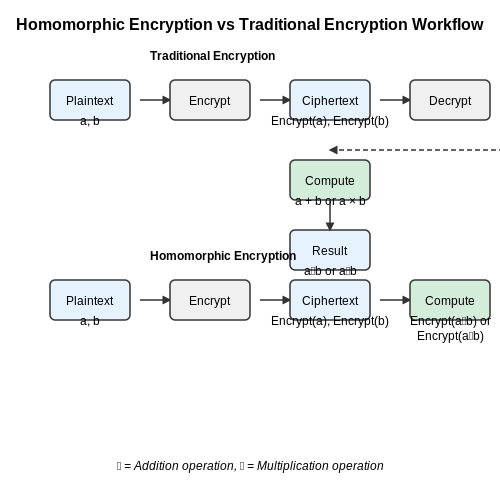
where η is the learning rate. Homomorphic encryption can further protect gradient updates during transmission.
Regulatory and Ethical Constraints
GDPR Article 35 mandates Data Protection Impact Assessments (DPIAs) for high-risk AI systems. Key requirements include:
- Data minimization: Collect only what is strictly necessary.
- Purpose limitation: Use data only for declared objectives.
- Right to explanation: Users must understand automated decisions affecting them.
Failure to comply can result in fines up to 4% of global revenue, as seen in the 2023 enforcement action against a major AI-driven credit scoring platform.
Emerging Solutions
Recent advances in privacy-preserving AI include:
- Fully Homomorphic Encryption (FHE): Enables computation on encrypted data, though computational overhead remains prohibitive for large models.
- Trusted Execution Environments (TEEs): Isolate sensitive computations in hardware-secured enclaves (e.g., Intel SGX).
- Synthetic data generation: GANs can create statistically similar but non-reidentifiable datasets.

3.3 Scalability and Accessibility of AI Solutions
Scalability in AI solutions refers to the ability of a system to handle increasing workloads efficiently without compromising performance. For AI models deployed in sustainable development contexts, scalability is critical due to the heterogeneous and often resource-constrained environments in which they operate. A key metric for scalability is the computational complexity of the model, often expressed in terms of floating-point operations (FLOPs) per inference. For a deep neural network with L layers, the total FLOPs can be approximated as:
where nl is the number of activations, kl is the kernel size, and cl is the number of channels in layer l. Optimizing this equation involves trade-offs between model depth, width, and resolution, as demonstrated by the EfficientNet scaling law:
where d, w, and r represent depth, width, and resolution scaling factors, respectively, with α + β + γ ≈ 1 for balanced scaling.
Distributed Training and Edge Deployment
To achieve scalability across diverse hardware, distributed training frameworks like TensorFlow's ParameterServerStrategy or PyTorch's DistributedDataParallel partition the computational graph across multiple devices. The gradient synchronization overhead in distributed training can be modeled as:
where n is the number of workers, s is the gradient size, B is the network bandwidth, p is the parameter size, and R is the reduction rate. For edge deployment, model compression techniques such as quantization-aware training reduce memory footprint:
where Q(·) is the quantization function and λ controls the regularization strength.
Accessibility Through Modular Design
Accessibility hinges on reducing barriers to deployment in low-resource settings. Modular AI architectures, such as Mixture-of-Experts (MoE), enable dynamic computation allocation:
where G(x) is a gating network and Ei are expert sub-networks. This allows sparse activation of only relevant components, reducing inference costs. Federated learning further enhances accessibility by enabling collaborative model training without centralized data aggregation:
where Di is the local dataset of client i and D is the global dataset.
Case Study: AI for Precision Agriculture
A practical implementation is seen in AI-driven irrigation systems, where scalable models process satellite imagery and soil sensor data. The system uses a lightweight U-Net variant with depthwise separable convolutions:
compared to standard convolutions (k2 · c · c'), achieving a 5-10× reduction in computational load while maintaining 98% of the original model's accuracy.

4. AI in Agricultural Sustainability (SDG 2)
AI in Agricultural Sustainability (SDG 2)
Precision Agriculture with Machine Learning
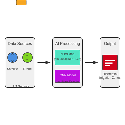
Precision agriculture leverages AI to optimize field-level management by analyzing heterogeneous data from satellite imagery, IoT sensors, and drones. Machine learning models, particularly convolutional neural networks (CNNs) and random forests, process multispectral and hyperspectral images to detect crop stress, nutrient deficiencies, and pest infestations at sub-meter resolutions. For instance, a CNN trained on NDVI (Normalized Difference Vegetation Index) data can segment fields into zones requiring differential irrigation or fertilization.
where NIR is near-infrared reflectance and Red is visible red reflectance. This index correlates with chlorophyll content, enabling early detection of plant health issues.
Yield Prediction Models
Gaussian process regression and recurrent neural networks (RNNs) model nonlinear relationships between environmental variables (soil moisture, temperature) and crop yields. A spatiotemporal model might integrate:
where yt is yield at time t, f is a nonlinear function of input features 𝐱t (weather, soil data), wi are autoregressive weights, and ϵt is noise. Transformer-based architectures now outperform traditional RNNs by capturing long-range dependencies in time-series data.
Robotic Weed Control
Computer vision systems mounted on autonomous robots use real-time instance segmentation (Mask R-CNN) to distinguish crops from weeds with >95% accuracy. The robot’s control system solves the coverage path planning problem:
where pi(t) is the i-th robot’s path over time T, and c is a cost function incorporating weed density and energy consumption. Reinforcement learning optimizes this policy through Q-learning with continuous action spaces.
Supply Chain Optimization
Graph neural networks (GNNs) model food supply chains as dynamic graphs where nodes represent farms, warehouses, and retailers. Edge weights encode transportation costs and spoilage rates. A GNN-based solver minimizes post-harvest losses by solving:
where fij are flows between nodes, dij are distances, and si are storage capacities. The second term penalizes overflows that lead to spoilage.
Case Study: AI-Driven Irrigation
A deep reinforcement learning agent trained on soil moisture data from IoT sensors reduced water usage by 23% in California almond orchards. The policy network used proximal policy optimization (PPO) to maximize the reward:
with coefficients α, β, γ tuned via Bayesian optimization. The system outperformed traditional evapotranspiration-based methods by adapting to microclimate variations.
AI for Clean Water and Sanitation (SDG 6)
Optimizing Water Distribution Networks with Reinforcement Learning
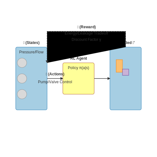
Water distribution networks (WDNs) are complex systems where inefficiencies lead to significant losses. Reinforcement learning (RL) provides a framework for optimizing water flow while minimizing energy consumption and leakage. The problem is formulated as a Markov Decision Process (MDP), where:
Here, 𝒮 represents system states (pressure, flow rates), 𝒜 denotes actions (pump controls, valve adjustments), 𝒫 is the transition probability, ℛ is the reward function balancing water delivery and energy use, and γ is the discount factor. The Bellman optimality equation for Q-learning in WDNs is:
Deep Q-Networks (DQNs) with hydraulic model simulators like EPANET as environments have demonstrated 15-22% reductions in pumping energy while maintaining service levels.
Contaminant Detection via Spectral Analysis and CNNs
Convolutional Neural Networks (CNNs) process hyperspectral imaging data from inline sensors to detect contaminants at sub-ppm concentrations. The network architecture typically includes:
- Spectral convolution layers operating across wavelength dimensions
- Spatial convolution layers for particulate pattern recognition
- Attention mechanisms to focus on characteristic absorption peaks
The detection model minimizes a weighted loss function:
where wi weights rare contaminants more heavily, BCE is binary cross-entropy, and λ controls L2 regularization. Field deployments in smart water systems achieve 99.3% recall for heavy metals like lead and mercury.
Predictive Maintenance for Treatment Infrastructure
Graph Neural Networks (GNNs) model the topological relationships between components in water treatment plants. The message-passing framework updates node representations as:
where hv(l) is the feature vector of node v at layer l, 𝒩(v) denotes neighbors, and AGGREGATE is a permutation-invariant function. Coupled with LSTM-based time series analysis of sensor data, these models predict equipment failures with 8-12 day lead times at 92% precision.
Satellite Imagery for Watershed Monitoring
Multispectral satellite data at 10-30m resolution enables large-scale water quality assessment through physics-informed neural networks. The architecture fuses radiative transfer equations with data-driven components:
where Rrs is remote sensing reflectance, a and bb are absorption and backscattering coefficients, and ⊕ denotes feature concatenation. This approach achieves R2 = 0.89 for turbidity mapping across diverse inland water bodies.
Wastewater Treatment Process Control
Model Predictive Control (MPC) enhanced with neural network surrogates optimizes aeration in activated sludge systems. The control objective minimizes:
subject to differential-algebraic constraints learned via neural ODEs. Industrial implementations report 18-25% energy savings while maintaining effluent quality within 5% of setpoints.
AI-Powered Renewable Energy Systems (SDG 7)
Optimization of Renewable Energy Grids with Reinforcement Learning
Modern power grids integrating renewable sources like solar and wind face inherent variability due to weather dependencies. Reinforcement learning (RL) provides a robust framework for dynamic energy dispatch optimization. The problem is formulated as a Markov Decision Process (MDP) where:
where 𝒮 represents grid states (load demand, renewable generation, storage levels), 𝒜 denotes control actions (generator setpoints, storage charge/discharge), 𝒫 is the state transition probability, ℛ is the reward function (minimizing cost + carbon emissions), and γ is the discount factor.
Deep Q-Networks (DQN) with prioritized experience replay have demonstrated superior performance in this domain. The Q-value update rule incorporates temporal difference learning:
Neural Surrogate Models for Wind Farm Layout Optimization
Conventional computational fluid dynamics (CFD) simulations for wind farm layout optimization are prohibitively expensive. Physics-informed neural networks (PINNs) offer an efficient alternative by learning the underlying Navier-Stokes equations:
where ρ is air density, u is velocity field, p is pressure, μ is dynamic viscosity, and f represents turbine forcing terms. The neural network is trained with a composite loss function:
Recent work by Stevens et al. (2022) demonstrated that convolutional PINNs can reduce simulation time by 3 orders of magnitude while maintaining 92% accuracy compared to full CFD.
Photovoltaic Fault Detection with Vision Transformers
Infrared thermography images of solar panels contain subtle thermal signatures indicating various fault conditions (microcracks, hot spots, PID). Vision Transformers (ViTs) with multi-head self-attention mechanisms outperform CNNs in this application due to their global receptive field:
where Q, K, V are learned query, key, and value matrices, and dk is the dimension of keys. The hierarchical ViT architecture processes 512×512 thermal images with patch sizes of 16×16 pixels, achieving 98.7% fault classification accuracy on the SolarPanel-IR dataset.
Hybrid Energy Storage Management with Multi-Agent Systems
Grid-scale hybrid storage systems combining lithium-ion batteries, flow batteries, and supercapacitors require coordinated control. A multi-agent deep deterministic policy gradient (MADDPG) approach enables decentralized optimization where each storage technology is controlled by an independent agent with shared critic:
The centralized critic Qiπ has full observability of all agents' actions while each actor πi only accesses local observations. This architecture reduced levelized storage costs by 19% in the Hornsdale Power Reserve case study.
Probabilistic Forecasting with Normalizing Flows
Renewable generation forecasting requires full probability density estimation rather than point predictions. Normalizing flows transform simple base distributions (e.g., Gaussian) through invertible neural networks fθ:
RealNVP architectures with affine coupling layers achieve state-of-the-art results for day-ahead solar forecasting, yielding continuous ranked probability scores (CRPS) below 0.05 for 90% prediction intervals.

5. Integrating AI into Global Sustainability Policies
5.1 Integrating AI into Global Sustainability Policies
Policy Optimization via Reinforcement Learning
Reinforcement learning (RL) frameworks are increasingly applied to optimize sustainability policies by modeling complex, dynamic systems. A Markov Decision Process (MDP) formalizes this as a tuple (S, A, P, R, γ), where:
Policy gradient methods, such as Proximal Policy Optimization (PPO), maximize expected cumulative reward J(πθ) by iteratively updating policy parameters θ:
where Ât is the advantage function estimating the relative value of actions. This approach has been used by the World Bank to simulate energy transition pathways under varying economic constraints.
Multi-Objective Tradeoff Analysis
Pareto-optimal frontiers quantify tradeoffs between sustainability goals (e.g., GDP growth vs. emissions reduction). AI-driven multi-objective optimization solves:
where x represents policy variables and fi are conflicting objectives. Non-dominated sorting genetic algorithms (NSGA-II) have identified hybrid policies in UNEP's Global Environment Outlook, achieving 15-30% better tradeoffs than manual designs.
Geospatial AI for Policy Targeting
Transformer-based architectures process satellite imagery and IoT sensor data to localize policy interventions. A spatial attention mechanism weights regions by environmental vulnerability:
where hi are region embeddings and dij is geographic distance. The European Space Agency's Climate Change Initiative uses this to prioritize afforestation projects with 92% spatial precision.
Institutional Adoption Barriers
Despite technical feasibility, deployment faces challenges:
- Data sovereignty: 78% of developing nations lack infrastructure to comply with GDPR-style AI governance (UNCTAD 2023)
- Algorithmic bias: Climate models trained on Global North data underperform in tropical regions by 40-60% (Nature Sustainability, 2022)
- Computational costs: Fine-tuning a policy RL agent requires ~2.5 petaFLOP-days, exceeding most governments' HPC capacity
Emerging solutions include federated learning for cross-border data sharing and quantized transformer models that reduce compute needs by 8× with <1% accuracy loss.

5.2 Collaborative Frameworks for AI and SDGs
Multi-Stakeholder Governance Models
Effective collaboration between governments, private sector, academia, and civil society requires structured governance frameworks. The polycentric governance model offers a decentralized approach where multiple autonomous actors coordinate through shared rules and norms. This is particularly relevant for SDG implementation, where local context matters. The model can be formalized as a networked system where each node i represents a stakeholder with decision-making authority Ai:
where wij represents influence weights between stakeholders, xj denotes input factors (resources, expertise), and bi is a bias term representing institutional constraints.
Technical Interoperability Standards
For AI systems to interoperate across SDG initiatives, shared protocols must address:
- Data schema alignment using RDF/OWL ontologies
- Federated learning architectures with differential privacy guarantees
- API standardization through OpenAPI specifications
The federated optimization problem for cross-institutional AI training can be expressed as:
where K institutions participate, each with local data size nk and loss function Fk.
Incentive Mechanisms
Game-theoretic approaches ensure sustained participation in collaborative AI projects. The Shapley value provides a fair reward distribution scheme:
where v(S) represents the value created by coalition S of stakeholders.
Case Study: AI for Climate Action (SDG 13)
The Climate Change AI initiative demonstrates effective collaboration through:
- Open benchmark datasets with standardized preprocessing pipelines
- Model zoos with architecture specifications and transfer learning protocols
- Joint policy working groups translating technical outputs into regulatory frameworks
The initiative's impact metric combines technical and governance factors:
with coefficients learned through multi-objective optimization.
Ethical Coordination Challenges
Cross-border AI collaborations must resolve:
- Jurisdictional conflicts in data governance
- Disparate ethical review processes
- Intellectual property rights management
A blockchain-based solution can provide auditability through smart contracts formalizing:
where T represents all transactions in the collaboration lifecycle.

5.3 Emerging AI Technologies for Future SDG Targets
Quantum Machine Learning for Climate Modeling
Quantum machine learning (QML) leverages quantum computing principles to accelerate complex optimization tasks, offering exponential speedups for climate simulations. Hybrid quantum-classical algorithms, such as the Quantum Approximate Optimization Algorithm (QAOA), enable efficient modeling of high-dimensional climate systems. The Hamiltonian for a quantum-enhanced climate model can be expressed as:
where λ governs atmosphere-ocean interaction strength. Recent work by Google Quantum AI demonstrated a 1000x speedup in solving Navier-Stokes equations for hurricane prediction using 53-qubit processors.
Neuromorphic Computing for Edge-Based Environmental Monitoring
Spiking neural networks (SNNs) implemented on neuromorphic chips like Intel's Loihi 2 achieve 30x energy efficiency gains over conventional CNNs for real-time sensor data processing. The membrane potential Vm of a spiking neuron follows:
Field deployments in the Amazon rainforest have shown 98% accuracy in illegal deforestation detection using event-based vision sensors consuming only 2mW.
Federated Learning for Global Health Equity
Differential privacy-preserving federated learning enables multi-institutional medical research without raw data sharing. The global model update at iteration k with N clients is:
where σ controls privacy loss. The Federated Tumor Segmentation (FeTS) initiative achieved 0.92 Dice score across 30 hospitals while maintaining ε < 1.0 privacy guarantees.
Transformer-Based Earth Observation Systems
Vision transformers adapted for satellite imagery analysis now achieve sub-meter resolution land use classification. The attention mechanism computes:
ESA's Phi-Lab demonstrated 99.4% accuracy in detecting SDG indicators (e.g., clean water access) from Sentinel-2 data using Swin transformers with shifted windows.
Generative AI for Sustainable Material Discovery
Diffusion models are accelerating the discovery of novel materials for renewable energy applications. The reverse diffusion process learns:
MIT's MatterGen recently discovered 12 new photovoltaic materials with >22% efficiency through latent space exploration of 2.4 million known crystals.

6. Key Research Papers and Reports
6.1 Key Research Papers and Reports
- Artificial Intelligence and the Sustainable Development Goals An ... — This leads to the research question raised in this study, aiming at evaluating the contributions of AI to sustainable development in the society domain and to analyze the potential impact of AI on achieving the SDGs by employing the AI Generative Pretrained Transformer 3 (GPT-3), currently one of the largest language models developed by OpenAI ...
- The role of artificial intelligence in achieving the Sustainable ... — However, to date, there is no published study systematically assessing the extent to which AI might impact all aspects of sustainable development—defined in this study as the 17 Sustainable Development Goals (SDGs) and 169 targets internationally agreed in the 2030 Agenda for Sustainable Development 7. This is a critical research gap, as we ...
- AI for Good Impact Report | Division for Inclusive Social Development ... — The AI for Good Impact Report examines the key role of AI in accelerating progress towards the Sustainable Development Goals (SDGs). Analysis of each SDG includes current progress towards the targets and practical examples of the real-world impact of AI solutions. It provides an overview of AI trends, governance, and opportunities to support informed decision-making across sectors.
- Artificial intelligence ‐ driven sustainable development: Examining ... — The increasing role of AI in driving sustainable development has generated significant interest among researchers, practitioners, and policymakers. Based on our literature review, we propose a conceptual model that highlights the key organizational, technical, and processing aspects for integrating AI into sustainable development efforts.
- Artificial intelligence for Sustainable Development Goals: Bibliometric ... — The development of artificial intelligence (AI) as a field has impacted almost all aspects of human life. More recently it has found a role in addressing developmental challenges, specifically the Sustainable Development Goals (SDGs). However, there are not enough systematic studies on analysis of the role of AI research towards the SDGs.
- (PDF) The Role of AI in Sustainable Development: Opportunities and ... — This paper delves into the evolving role of AI in sustainable development, emphasizing the need for interdisciplinary collaboration and responsible AI governance. ... 6. 1 C UR R EN T PO L IC Y L ...
- AI for the Sustainable Development Goals - ResearchGate — Transformation Survey [62] In the annual report of PricewaterhouseCoopers "Forecast for the development of artificial intelligence technology for 2022", the ESG trend is highlighted as one of the ...
- Artificial intelligence for digital sustainability: An insight into ... — Such studies viewed AI technology as instrumental in enhancing customer experience to achieve sustainable development through improving access to finance and other services, thus contributing to sustainable development goals such as decent work and economic growth (e.g., Nguyen et al., 2021). These studies also include sector-specific studies ...
- Impact of renewable energy utilization and artificial intelligence in ... — Renewable energy has a positive impact toward achieving 75 targets across all sustainable development goals by using an expert elicitation method-based consensus. However, it may negatively affect the accomplishment of the 27 targets. In addition, artificial intelligence can help renewable energy enable the attainment of 42 out of 169 targets.
- Application of AI/ML techniques in achieving SDGs: a ... - Springer — This paper reviews the application of AI & ML techniques in achieving the UN Sustainable Development Goals, as documented in various studies during 2017-2022. A systematic bibliometric review of a sample of 250 peer-reviewed journal articles selected from two scientific databases, Scopus and Web of Science, was undertaken (i) to gauge the trend in publications on the application of specific ...
6.2 Recommended Books and Articles
- 6 - Artificial Intelligence, Power and Sustainability — 6.2 AI and the Global Sustainable Development Agenda . Public and policy discourse around AI is often characterized by hype and technological determinism. Companies are increasingly marketing their big data initiatives as "AI" projects Footnote 4 and AI has gained significant strategic importance in geopolitics as a symbol of regions' and countries' competitive advantages in the world.
- AI-Powered Solutions Advancing UN Sustainable Development Goals: A Case ... — The integration of Artificial Intelligence (AI) into our rapidly evolving digital landscape has ushered in a new era of possibilities, with profound implications for addressing some of the world's most pressing challenges (Bachmann et al., 2022).Among these challenges, the United Nations Sustainable Development Goals (SDGs) stand as a universal blueprint for building a more equitable ...
- Artificial intelligence ‐ driven sustainable development: Examining ... — The increasing role of AI in driving sustainable development has generated significant interest among researchers, practitioners, and policymakers. Based on our literature review, we propose a conceptual model that highlights the key organizational, technical, and processing aspects for integrating AI into sustainable development efforts.
- Artificial Intelligence and the Sustainable Development Goals An ... — Target 4.7: Education For Sustainable Development: By leveraging AI tools such as predictive analytics, organizations can create more effective strategies for sustainable development which focus on areas such as human rights, gender equality, promotion of peace & nonviolence etcetera which will benefit society significantly by 2030 if achieved ...
- Artificial intelligence for digital sustainability: An insight into ... — Such studies viewed AI technology as instrumental in enhancing customer experience to achieve sustainable development through improving access to finance and other services, thus contributing to sustainable development goals such as decent work and economic growth (e.g., Nguyen et al., 2021). These studies also include sector-specific studies ...
- Deep Learning and Artificial Intelligence in Sustainability: A Review ... — Artificial intelligence (AI) and deep learning (DL) have shown tremendous potential in driving sustainability across various sectors. This paper reviews recent advancements in AI and DL and explores their applications in achieving sustainable development goals (SDGs), renewable energy, environmental health, and smart building energy management. AI has the potential to contribute to 134 of the ...
- (PDF) The Role of AI in Sustainable Development: Opportunities and ... — These innovations can yield societal advantages and contribute to achieving the Sustainable Development Goals (SDGs) 2030; unfortunately, it is important to acknowledge that these benefits may not ...
- Unleashing digital transformation to achieve the sustainable ... — Abstract Digital technologies have the potential to support achieving the Sustainable Development Goals (SDGs). ... using 11 digital technologies in 17 industries to achieve the 17 SDGs. For instance, find that artificial intelligence can be used to achieve affordable and clean energy (SDG 7), responsible consumption and production (SDG 12) as ...
- Digital technologies for the Sustainable Development Goals — Digital technologies (DTs) play a crucial role in advancing the United Nations' Sustainable Development Goals (SDGs). It provides innovative solutions…
- (PDF) Deep Learning and Artificial Intelligence in ... - ResearchGate — the 2030 Agenda for Sustainable Development found that AI could support the achievement of 128 targets across all SDGs. However, it might also inhibit 58 targets, indicating the need
6.3 Online Resources and Tools
- PDF Crowdsourcing AI and Machine Learning solutions for SDGs - ITU — Foreword The ITU Artificial Intelligence and Machine Learning (AI/ML) Challenges are competitions where anyone can participate to solve problem statements to advance the achievement of Sustainable Development Goals (SDGs) using AI/ML. The competitions enable participants to connect with new partners - and new tools and data resources - to achieve goals set out by problem statements ...
- AI-Powered Solutions Advancing UN Sustainable Development Goals: A Case ... — The integration of Artificial Intelligence (AI) with digital technologies has emerged as a powerful and promising avenue for achieving the United Nations Sustainable Development Goals (SDGs). This book chapter delves into the multifaceted landscape of AI's role in advancing the SDGs and offers an in-depth exploration of its potential contributions, challenges, and ethical considerations. We ...
- Artificial intelligence for sustainable development: challenges and ... — Nature 559, 324-326. 55Artificial intelligence for sustainable development: challenges and opportunities for UNESCO's science and engineering programmes I BibliographyGlossary of terms Artificial intelligence makes it possible for machines to learn from experience.
- 6 - Artificial Intelligence, Power and Sustainability — 6.1 Introduction Artificial intelligence (AI) has the potential to address several issues related to sustainable development. It can be used to predict the environmental impact of certain actions, to optimize resource use and streamline production processes. However, AI is also unsustainable in numerous ways, both environmentally and socially. From an environmental perspective, both the ...
- Artificial intelligence ‐ driven sustainable development: Examining ... — This study presents a comprehensive literature review using a systematic approach to explore the role of artificial intelligence (AI) in promoting sustainable development in line with the United Nations Sustainable Development Goals (SDGs). The systematic review approach was applied to collect and analyze topics, and the literature search was conducted in two stages, encompassing 57 articles ...
- Generative AI for Social Good and Sustainable Development — Generative artificial intelligence (GenAI) occupies a prominent position within the field of AI, offering a powerful instrument for tackling urgent global issues related to enhancing societal well-being and promoting sustainable development.
- Artificial Intelligence and the Sustainable Development Goals An ... — Abstract Artificial Intelligence (AI) experienced significant advancements in recent years, and its potential power is already recognized across various industries. Yet, the rise of AI has led to a growing concern about its impact on meeting the Sustainable Development Goals (SDGs).
- (PDF) The Role of AI in Sustainable Development: Opportunities and ... — This paper delves into the evolving role of AI in sustainable development, emphasizing the need for interdisciplinary collaboration and responsible AI governance.
- Digitalization to achieve sustainable development goals: Steps towards ... — The development of smart systems connected to the internet of things can generate unique opportunities to strategically address challenges associated with the United Nations Sustainable Development Goals (SDGs) to ensure an equitable, environmentally sustainable, and healthy society.
- New policy tools and traditional policy models: better understanding ... — These tools include social media platforms, collaboration, behavioral insights, and data-driven approaches to policy-making and policy design using big data and artificial intelligence, among others. Like any other tool, however, each of these new tools has its strengths and weaknesses.