Reasoning on Structured and Semi-Structured Data
1. Definition and Key Characteristics
Definition and Key Characteristics
Structured data adheres to a rigid schema, typically represented in relational databases, spreadsheets, or matrices, where each entry conforms to predefined fields. Semi-structured data, while lacking a fixed schema, contains self-describing markers such as tags (XML, JSON) or key-value pairs (NoSQL databases), enabling partial organization without strict relational constraints.
Formal Representation
Structured data can be modeled as a relational tuple R(A₁, A₂, ..., Aₙ), where attributes Aᵢ enforce domain constraints. For semi-structured data, the model becomes a labeled graph G = (V, E, L), where vertices V represent entities, edges E denote relationships, and labels L provide metadata.
Key Characteristics
- Schema Enforcement: Structured data requires upfront schema definition (DDL in SQL), while semi-structured permits schema-on-read (e.g., MongoDB's BSON).
- Query Complexity: Structured data enables efficient joins via foreign keys, whereas semi-structured traversals require path queries (XPath, Gremlin).
- Flexibility Trade-off: Semi-structured formats like JSON tolerate heterogeneous nested data but sacrifice optimization opportunities (columnar storage, indexing).
Information Extraction Challenges
Reasoning over semi-structured data demands probabilistic schema inference. For a JSON document D with nested objects, type inference becomes:
where τ is the inferred type and vₖ the value at key k. Modern systems like Apache Spark use sampling-based schema detection.
Case Study: Biomedical Data Integration
Clinical trials (structured) often integrate with EHRs (semi-structured JSON/HL7). A federated query across both requires:
- Schema mapping between ICD-10 codes (structured) and physician notes (unstructured annotations in JSON)
- Graph-based linkage of patient IDs to trial participants via probabilistic record matching
Common Formats: JSON, XML, CSV, and Relational Databases
JSON (JavaScript Object Notation)
JSON is a lightweight, text-based data interchange format that uses human-readable text to store and transmit structured data. It is built on two primary structures: a collection of key-value pairs (objects) and an ordered list of values (arrays). JSON's syntax is derived from JavaScript but is language-independent, making it widely adopted in web APIs and NoSQL databases like MongoDB.
Its schema-less nature allows flexibility, but validation tools like JSON Schema enforce structure when needed. JSON is efficient for nested data but lacks native support for binary data, often requiring Base64 encoding.
XML (eXtensible Markup Language)
XML is a markup language that defines rules for encoding documents in a format that is both human-readable and machine-readable. Unlike JSON, XML supports metadata via attributes and namespaces, enabling complex document structures with mixed content. Its hierarchical tree structure is governed by Document Type Definitions (DTD) or XML Schema (XSD).
XML's verbosity increases parsing overhead, but its validation capabilities make it dominant in enterprise systems (e.g., SOAP web services) and document formats like Office Open XML.
CSV (Comma-Separated Values)
CSV is a delimited text format where each line represents a record, and commas separate fields. Despite its simplicity, CSV lacks standardization: escaping rules, line breaks, and headers vary across implementations. Pandas and Apache Commons CSV handle edge cases like quoted delimiters or multiline fields.
Optimized for tabular data, CSV struggles with hierarchical relationships, often requiring flattening or multiple files linked by keys.
Relational Databases
Relational databases (e.g., PostgreSQL, MySQL) store data in normalized tables with rows and columns, enforcing integrity via ACID transactions. SQL queries join tables using primary/foreign keys, optimizing for OLTP workloads. The relational model minimizes redundancy but requires upfront schema design.
Indexes (B-trees, hash) accelerate lookups, while views and stored procedures abstract complexity. ORMs like SQLAlchemy bridge object-oriented code and relational schemas.
Comparative Analysis
- Schema Flexibility: JSON/XML allow dynamic structures; CSV/relational databases require predefined schemas.
- Query Capabilities: SQL offers declarative querying; JSON/XML rely on XPath, JSONPath, or manual traversal.
- Performance: Binary formats (Protocol Buffers, Avro) outperform text-based JSON/XML/CSV in serialization speed.
Hybrid systems like PostgreSQL's JSONB column type combine relational rigor with document flexibility, enabling queries like SELECT * FROM table WHERE data->>'key' = 'value'.
1.3 Differences Between Structured and Semi-Structured Data
Structured data adheres to a rigid schema, enforcing a predefined model where data types, relationships, and constraints are explicitly defined. Relational databases exemplify this paradigm, storing data in tables with fixed columns and datatypes, enabling efficient querying via SQL. The schema-on-write approach ensures validation occurs before ingestion, guaranteeing consistency. For instance, a customer database might enforce NOT NULL constraints on primary keys and foreign key relationships between orders and products.
Schema Flexibility and Evolution
Semi-structured data lacks a fixed schema, instead employing self-describing formats like JSON, XML, or YAML that embed metadata within the payload. This schema-on-read model defers validation until access, accommodating heterogeneous or evolving data. Consider a sensor network emitting JSON records: new fields can appear dynamically without schema migrations, but queries must handle missing or inconsistent fields. The trade-off manifests in storage efficiency versus adaptability—structured data optimizes for query performance while semi-structured prioritizes flexibility.
Query Capabilities and Performance
Structured systems enable complex joins and ACID transactions through query optimizers that leverage schema knowledge. The explicit relationships allow cost-based optimizers to select efficient execution plans. In contrast, semi-structured systems often require denormalization or nested structures, pushing filtering logic to application code. GraphQL and JSONPath emerge as query languages for semi-structured data, but lack the algebraic foundations of relational algebra underpinning SQL. Performance diverges significantly at scale: analytical queries on structured data can exploit columnar storage and indexing, while semi-structured systems may require full scans or specialized indexes like inverted indices.
Typical Use Cases
- Structured: Financial systems (transaction integrity), inventory management (strict schemas), reporting (aggregation over known dimensions)
- Semi-structured: Log analysis (evolving fields), IoT (heterogeneous devices), web APIs (version-tolerant payloads)
Formal Modeling Differences
Structured data maps to relational algebra's tuples and relations, where domains (data types) and constraints are explicit. Semi-structured data aligns with graph models—trees (JSON/XML) or property graphs—where edges can carry attributes. The absence of a global schema complicates formal verification; type systems for semi-structured data employ gradual typing or schema languages like JSON Schema that provide partial validation.
2. Query Languages (SQL, SPARQL)
Query Languages (SQL, SPARQL)
Relational Querying with SQL
SQL (Structured Query Language) is the de facto standard for querying relational databases. Its declarative syntax allows users to retrieve, manipulate, and transform structured data without specifying procedural steps. The core operations—selection (SELECT), projection (WHERE), joins (JOIN), and aggregation (GROUP BY)—form a relational algebra foundation.
For complex analytical queries, window functions extend SQL’s capabilities:
This computes a rank for each row within a partition, enabling operations like running totals or moving averages without collapsing rows. Modern SQL engines (PostgreSQL, DuckDB) also support recursive queries via Common Table Expressions (CTEs), allowing traversal of hierarchical data:
WITH RECURSIVE tree_path AS (
  SELECT id, parent_id, name FROM nodes WHERE id = 1
  UNION ALL
  SELECT n.id, n.parent_id, n.name FROM nodes n
  JOIN tree_path tp ON n.parent_id = tp.id
) SELECT * FROM tree_path;
Graph Querying with SPARQL
SPARQL (SPARQL Protocol and RDF Query Language) operates on RDF (Resource Description Framework) graphs, where data is represented as triples (subject-predicate-object). Its pattern-matching syntax aligns with graph traversal:
SELECT ?person WHERE {
  ?person foaf:knows ?friend .
  ?friend foaf:interest "AI" .
}
SPARQL’s OPTIONAL operator handles missing data gracefully, unlike SQL’s strict joins. Property paths (foaf:knows+) enable transitive closures for recursive relationships. For federated queries across distributed RDF datasets, SERVICE clauses delegate subqueries to remote endpoints.
Comparative Semantics
SQL and SPARQL differ fundamentally in their data models and execution strategies:
- Joins vs. Triple Patterns: SQL optimizes tabular joins via cost-based planners, while SPARQL uses graph pattern matching with index nested loops.
- Null Handling: SQL’s three-valued logic (true/false/unknown) contrasts with SPARQL’s unbound variables in solution mappings.
- Set vs. Bag Semantics: SQL defaults to bag semantics (duplicates allowed), whereas SPARQL results are sets unless
DISTINCTis omitted.
Hybrid systems like Apache Jena’s SDB bridge this gap by translating SPARQL to SQL for relational backends, leveraging existing query optimizers.
Performance Considerations
Query planning in both languages benefits from statistical summaries—histograms in SQL, RDF stats like predicate frequency in SPARQL. For example, a selectivity estimate for a triple pattern {?s p ?o} is derived from:
Materialized views (SQL) or precomputed RDF molecules (SPARQL) accelerate repetitive analytical queries. Modern engines like Trino and Blazegraph use vectorized execution and caching to mitigate latency in federated scenarios.

2.2 Rule-Based Reasoning and Deductive Databases
Rule-based reasoning systems operate on formal logic principles, where knowledge is represented as a set of if-then rules and facts. These systems derive conclusions through forward or backward chaining, making them particularly effective for structured and semi-structured data where relationships can be explicitly defined. Deductive databases extend traditional relational databases by integrating logical inference capabilities, enabling query answering through rule application.
Logical Foundations
The core of rule-based reasoning lies in first-order logic (FOL), where rules take the form:
Here, P(X) is the antecedent (body) and Q(X) the consequent (head). A deductive database consists of:
- Extensional Database (EDB): Base facts stored as ground atoms (e.g., employee(john, engineering)).
- Intensional Database (IDB): Rules defining derived predicates (e.g., department_head(X) ← employee(X, Y), manager(X, Y)).
Inference Mechanisms
Two primary inference strategies are employed:
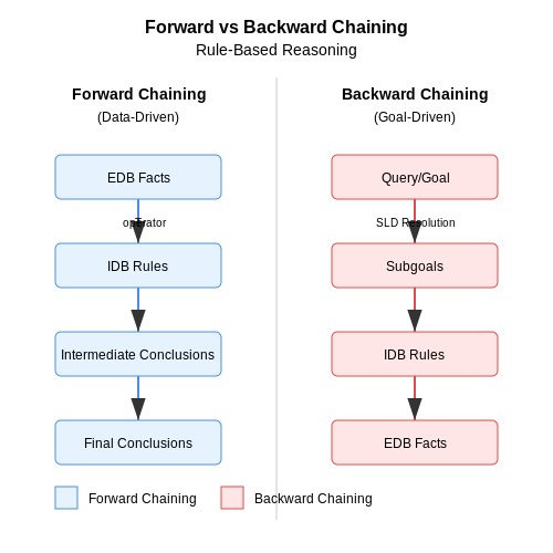
Forward Chaining (Bottom-Up)
Starting from known facts, the system applies rules iteratively until no new conclusions can be drawn. This approach is data-driven and computes the minimal model of the database. The fixpoint iteration is formalized as:
where I is the current interpretation and TP the immediate consequence operator.
Backward Chaining (Top-Down)
Goal-directed reasoning starts from a query and recursively decomposes it using IDB rules until it reaches EDB facts. This is implemented via SLD resolution in Prolog-like systems.
Datalog: A Deductive Database Language
Datalog restricts FOL to ensure decidability and efficient evaluation. Key features include:
- Range-restricted variables (all variables in the head must appear in the body).
- Negation-as-failure under stratified semantics.
- No function symbols to guarantee termination.
Example Datalog program:
ancestor(X, Y) :- parent(X, Y).
ancestor(X, Y) :- parent(X, Z), ancestor(Z, Y).
Optimization Techniques
Efficient evaluation requires:
- Magic Sets: Rewrites rules to simulate top-down evaluation in a bottom-up system, pushing query constraints into rule bodies.
- Join Ordering: Reorders body literals to minimize intermediate relation sizes.
- Incremental View Maintenance: Updates materialized views incrementally when EDB changes.
Applications
Rule-based reasoning powers:
- Enterprise Policy Systems: Enforcing compliance rules over organizational data.
- Semantic Web: OWL reasoning via rule-based entailment regimes.
- Network Security: Real-time intrusion detection using event-condition-action rules.
Graph-Based Reasoning (Property Graphs, RDF)
Property Graphs: Structure and Querying
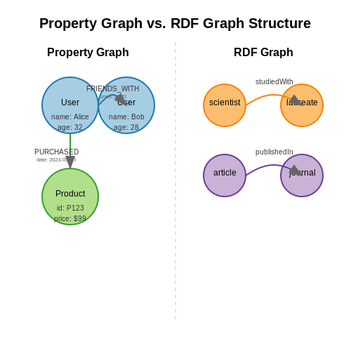
Property graphs model data as nodes (vertices) connected by edges (relationships), where both nodes and edges can have key-value attributes. Formally, a property graph G is defined as a tuple:
where V is the set of vertices, E is the set of edges, λ assigns labels to nodes and edges, and ρ assigns properties (key-value pairs). This model excels in traversal efficiency, making it ideal for social networks, recommendation systems, and fraud detection.
Cypher, the query language for Neo4j, enables expressive pattern matching. For example, finding mutual friends between two users:
MATCH (a:User)-[:FRIENDS_WITH]->(mutual:User)<-[:FRIENDS_WITH]-(b:User)
WHERE a.id = 'Alice' AND b.id = 'Bob'
RETURN mutual.name
RDF and Semantic Reasoning
Resource Description Framework (RDF) represents data as triples (subject, predicate, object), enabling formal semantics through ontologies like OWL. An RDF graph is a set of triples:
where U is URIs, B is blank nodes, and L is literals. SPARQL queries leverage graph patterns, such as this query for scientists who studied with a Nobel laureate:
PREFIX nobel: <http://example.org/nobel>
SELECT ?scientist WHERE {
    ?laureate a nobel:Laureate .
    ?scientist nobel:studiedWith ?laureate .
}
Inference in Graph Databases
RDF supports rule-based reasoning via RDFS and OWL entailment. For instance, subclass relationships propagate through transitive rules:
Property graphs achieve inference through procedural traversals, such as calculating PageRank for node importance:
where d is a damping factor, Bu is the set of nodes linking to u, and L(v) is the out-degree of v.
Performance Tradeoffs
Property graphs optimize for low-latency traversals (O(1) edge lookups via adjacency lists), while RDF systems leverage triple-store indices (e.g., Hexastore) for complex SPARQL joins. Benchmarks show Neo4j outperforms RDF stores in neighbor queries by 10–100x, but RDF engines like Virtuoso handle federated queries across distributed datasets more efficiently.
3. Schema Inference and Data Wrangling
Schema Inference and Data Wrangling
Schema inference is the process of automatically detecting the structure of structured or semi-structured data, such as JSON, XML, or relational tables, without explicit schema definitions. This is critical for integrating heterogeneous data sources, where manual schema specification is impractical. Probabilistic graphical models, such as Hidden Markov Models (HMMs) or Conditional Random Fields (CRFs), are often employed to infer hierarchical relationships and data types.
Probabilistic Schema Inference
Given a dataset D with n records, the goal is to infer a schema S that maximizes the likelihood P(S|D). Using Bayesian inference, we compute:
where P(D|S) is the likelihood of the data given the schema, and P(S) is the prior probability of the schema. For semi-structured data, a common approach is to model schema inference as a tree-structured problem, where nodes represent fields and edges denote hierarchical dependencies.
Data Wrangling with Schema Alignment
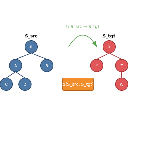
Once a schema is inferred, data wrangling involves transforming raw data into a consistent format. Schema alignment resolves structural mismatches between inferred and target schemas. Let Ssrc and Stgt be source and target schemas, respectively. The alignment function f: Ssrc → Stgt minimizes the dissimilarity metric:
where wi are weights for different schema attributes (e.g., field names, data types), and d is a distance function (e.g., Jaccard similarity for categorical fields, Euclidean distance for numerical ranges).
Practical Applications
In enterprise data lakes, automated schema inference enables dynamic ingestion of JSON logs or CSV files without predefined templates. For example, a financial institution aggregating transaction records from multiple banks can use probabilistic schema matching to align "transaction_date" (source) with "date_of_transaction" (target). Graph-based alignment algorithms, such as Gromov-Wasserstein optimal transport, improve matching accuracy for nested structures.
Handling Noisy and Missing Data
Real-world datasets often contain missing values or inconsistent entries. Imputation techniques, such as Gaussian Process Regression (GPR) for numerical fields or Bayesian Multinomial Models for categorical data, can be applied after schema inference. For a field X with missing values, the imputed value X̂ is derived from:
where the expectation is conditioned on observed values and the inferred schema constraints.
3.2 Path-Based Querying (XPath, JSONPath)
Path Querying Fundamentals
Path-based querying enables precise traversal and extraction of data from hierarchical structures like XML and JSON. XPath and JSONPath are domain-specific languages (DSLs) designed for this purpose, operating on tree-like representations of structured documents. Both languages use path expressions to navigate nodes, with syntax optimized for filtering, conditional selection, and recursive descent.
XPath: XML Path Language
XPath 3.1, the latest W3C standard, provides a rich set of axes (child::, parent::, descendant::), node tests (element, attribute, text), and predicates. The location path /bookstore/book[price>35]/title demonstrates:
- Absolute path starting from root (
/bookstore) - Child axis selection (
/book) - Predicate filtering (
[price>35])
XPath Axes and Functions
Advanced XPath leverages axes for contextual navigation:
//employee[ancestor::department[@id='engineering']]/name[string-length() > 5]This query combines:
- Recursive descent (
//employee) - Axis-based ancestor filtering
- String function predicate
JSONPath for Semi-Structured Data
JSONPath adapts XPath concepts for JSON, using JavaScript-like syntax. The expression $$.store.book[?(@.price < 10)].title selects book titles where price is below 10. Key operators include:
- $$ - Root object
- . - Child member
- [] - Subscript operator
- ?() - Filter expression
JSONPath Execution Semantics
JSONPath evaluation follows formal grammar rules:
Where child is a JSON key and F is a filter expression. Implementations vary in support for recursive descent (..) and script expressions.
Performance Considerations
Path query engines optimize using:
- Precompiled path patterns - Convert expressions to deterministic finite automata (DFA)
- Lazy evaluation - Defer computation of branches until needed
- Index acceleration - Map common paths to B-tree or hash indexes
Where k is path length and d is average node depth. Modern processors achieve throughput of 106 queries/sec on indexed datasets.
Real-World Implementations
Production systems combine path querying with other paradigms:
// MongoDB aggregation with JSONPath-like syntax
db.inventory.aggregate([
  { $$match: { "items": { $$elemMatch: { price: { $$lt: 20 } } } }
])3.3 Probabilistic and Fuzzy Reasoning Approaches
Probabilistic reasoning provides a framework for handling uncertainty in structured and semi-structured data by modeling likelihoods using probability theory. Bayesian networks, a key tool in this domain, represent variables as nodes and conditional dependencies as directed edges. The joint probability distribution over n variables decomposes as:
where Parents(Xi) denotes the direct dependencies of Xi. Inference in Bayesian networks typically involves message-passing algorithms like belief propagation, which computes marginal distributions by passing local messages between nodes. For tree-structured networks, exact inference is tractable, but for general graphs, approximate methods like Markov Chain Monte Carlo (MCMC) sampling become necessary.
Fuzzy logic extends probabilistic reasoning by introducing degrees of truth through membership functions. A fuzzy set A in universe X is characterized by:
where μA(x) quantifies the degree to which x belongs to A. Fuzzy reasoning operates through composition rules, most commonly using Zadeh's extension principle for mapping fuzzy inputs through functions. The Mamdani inference system, widely used in control applications, executes fuzzy reasoning in four steps: fuzzification, rule evaluation, aggregation, and defuzzification (often using centroid methods).
Hybrid Probabilistic-Fuzzy Systems
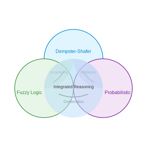
Advanced reasoning systems combine probabilistic and fuzzy approaches to handle both stochastic uncertainty and linguistic vagueness. The Dempster-Shafer theory provides a mathematical framework for such integration, where basic probability assignments distribute belief masses across power sets:
where Θ is the frame of discernment. Combining evidence from multiple sources uses Dempster's rule of combination:
Practical implementations often employ probabilistic fuzzy rule bases, where each rule Ri takes the form:
where CF represents the certainty factor as a probability measure. These systems excel in medical diagnosis and industrial process control where both sensor noise (probabilistic) and expert knowledge (fuzzy) must be reconciled.
Markov Logic Networks
For relational data, Markov Logic Networks (MLNs) unify probabilistic graphical models with first-order logic. An MLN consists of weighted first-order formulas, where each grounding forms a feature in a Markov network. The probability of a possible world x is given by:
where wi are formula weights, ni(x) counts true groundings, and Z is the partition function. Inference in MLNs uses techniques like MaxWalkSat for MAP estimates or MC-SAT for marginal probabilities, enabling reasoning over structured knowledge bases with uncertain rules.
4. Embedding-Based Methods for Structured Data
4.1 Embedding-Based Methods for Structured Data
Embedding-based methods transform structured and semi-structured data into continuous vector spaces, enabling machine learning models to process relational and hierarchical information efficiently. These techniques are particularly powerful for tasks like knowledge graph completion, tabular data reasoning, and schema matching.
Relational Embeddings for Tabular Data
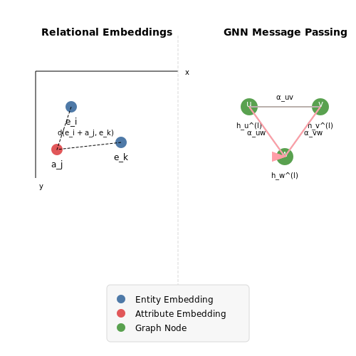
Relational embeddings capture the semantic relationships between entities in structured tables. Given a table with rows as entities and columns as attributes, we can learn embeddings for both entities and attributes. The key idea is to minimize a distance metric between related entities while maximizing separation for unrelated ones.
where ei, ek, el are entity embeddings, aj is an attribute embedding, d is a distance function (typically L2 norm), and γ is a margin hyperparameter. The triplet (ei,aj,ek) indicates that attribute aj relates entity ei to ek.
Graph Neural Networks for Structured Representations
Graph Neural Networks (GNNs) extend embedding approaches to explicitly model graph-structured data. For a knowledge graph G = (V,E) with nodes v ∈ V and edges e ∈ E, a GNN computes node embeddings through iterative message passing:
where hv(l) is the embedding of node v at layer l, N(v) denotes neighbors of v, and AGGREGATE is a permutation-invariant function (e.g., mean, max, or attention-based pooling). The final node embeddings capture both local graph structure and global relational patterns.
Attention Mechanisms for Heterogeneous Data
When dealing with semi-structured data containing multiple relation types (e.g., knowledge graphs with different edge types), attention mechanisms weight the importance of different relations dynamically. The attention coefficient αuv between nodes u and v with relation r is computed as:
where a is a learnable attention vector, W and Wr are weight matrices, and ∥ denotes concatenation. This allows the model to focus on the most relevant relations when aggregating information.
Practical Applications
- Knowledge Graph Completion: Embedding methods predict missing links in knowledge graphs by scoring candidate triples using learned embeddings.
- Semantic Table Interpretation: Embeddings enable matching columns across tables by comparing their vector representations in a shared space.
- Recommendation Systems: User-item interactions in relational databases are modeled through joint embeddings of users, items, and their attributes.
Recent advances like Transformer-based architectures have further improved these methods by enabling contextualized embeddings that adapt to the surrounding data structure. For instance, TaBERT (Yin et al., 2020) learns joint representations of tables and text by encoding both the table structure and surrounding natural language context.
4.2 Neural-Symbolic Integration
Neural-symbolic integration combines the strengths of neural networks (sub-symbolic learning) and symbolic reasoning (logic-based systems) to create models capable of learning from data while retaining interpretability and logical consistency. This hybrid approach addresses key limitations of purely neural or purely symbolic systems, such as the lack of explainability in deep learning and the brittleness of hand-crafted symbolic rules.
Architectural Paradigms
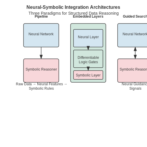
Three primary architectures dominate neural-symbolic integration:
- Neural-Symbolic Pipeline: Neural networks preprocess raw data into symbolic representations, which are then fed to a symbolic reasoner. For example, object detection followed by logical rule application.
- Embedded Symbolic Layers: Differentiable implementations of symbolic operations (e.g., logic gates, constraint solvers) are inserted as layers within neural networks.
- Neural-Guided Symbolic Search: Neural networks guide the search process in symbolic systems, such as in theorem proving or program synthesis.
Differentiable Logic Programming
A key innovation enabling tight integration is the development of differentiable logic operators. Consider a first-order logic rule:
This can be made differentiable by interpreting logical operations as fuzzy set operations. For example, the implication P ⇒ Q becomes:
where P and Q are continuous truth values in [0,1]. This allows gradient-based optimization while preserving logical semantics.
Neural Theorem Proving
Modern systems like Neural Logic Machines implement differentiable forward chaining. Given a set of Horn clauses and facts, the system computes:
where T is the set of derived facts and R is the set of rules. The neural component learns rule weights and fact embeddings, enabling soft matching of symbolic patterns.
Case Study: Visual Question Answering
In visual QA systems, neural-symbolic integration enables compositional reasoning. The pipeline:
- A CNN processes the image into object embeddings
- A transformer parses the question into a logical form
- A differentiable prover executes the query over the scene graph
For the question "Is there a red block to the left of a blue sphere?", the system might learn to execute:
where all predicates are implemented as neural modules with differentiable semantics.
Challenges and Frontiers
Current research focuses on:
- Scaling to more complex logics (higher-order, modal)
- Handling uncertainty in symbolic operations
- Joint learning of neural representations and symbolic rules
- Verification of integrated systems
The field continues to evolve with architectures like DeepProbLog and Neurosymbolic Concept Learners pushing the boundaries of integrated reasoning.
4.3 Transformer Models for Semi-Structured Data
Transformer architectures, originally designed for sequential text data, have been adapted to handle semi-structured data such as JSON, XML, and tabular formats. The key challenge lies in preserving hierarchical relationships while leveraging self-attention mechanisms. Unlike traditional NLP tasks, semi-structured data requires specialized tokenization and positional encoding strategies to capture nested dependencies.
Tokenization Strategies for Hierarchical Data
Standard subword tokenization (e.g., WordPiece, Byte-Pair Encoding) fails to preserve structural boundaries in nested formats. Modified approaches include:
- Path-based tokenization: Encodes elements with full XPath/JSONPath identifiers (e.g., /root/items[3]/price)
- Structural markers: Inject special tokens for opening/closing tags and nesting levels
- Graph-based segmentation: Treats data as a directed acyclic graph with edge-aware attention
Extended Attention Mechanisms
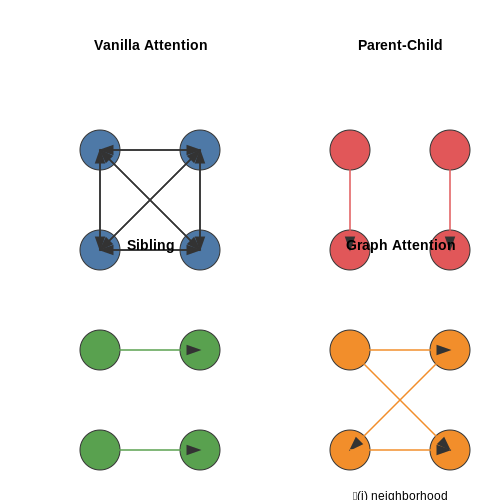
Vanilla self-attention computes relationships between all tokens equally. For semi-structured data, constrained attention patterns improve performance:
Where 𝒩(i) defines the neighborhood of token i based on structural relationships. Common variants include:
- Parent-child attention: Only allows attention between opening/closing tags and their contents
- Sibling attention: Restricts attention to elements at the same nesting level
- Graph attention: Uses predefined schema edges as attention pathways
Relative Positional Encoding
Standard sinusoidal positional encoding fails to capture tree-like structures. Tree positional encodings incorporate:
Where TreeDistance measures the shortest path between nodes in the parse tree. Implementations often use learnable parameters for each relative position type (ancestor, descendant, sibling).
Schema-Aware Pretraining
Modern architectures like TAPAS (Google) and RAT-SQL extend BERT-style pretraining with:
- Masked schema modeling: Randomly masks column/field names and predicts from values
- Structural alignment loss: Penalizes attention weights that cross schema boundaries
- Path prediction: Trains the model to reconstruct element access paths
These models achieve state-of-the-art results on benchmarks like Spider (text-to-SQL) and WebNLG (data-to-text generation), with schema-aware variants outperforming vanilla transformers by 15-30% on exact match metrics.
Case Study: Table Transformer (Microsoft)
The TaBERT architecture processes relational tables through:
- Vertical attention heads that operate across table columns
- Horizontal attention restricted to rows
- Special [HEADER] tokens that attend to all cells in their column
This achieves 92.1% accuracy on WikiTableQuestions while reducing compute costs by 40% compared to full attention over flattened table representations.
5. Knowledge Graphs and Semantic Web
Knowledge Graphs and Semantic Web
Foundations of Knowledge Graphs
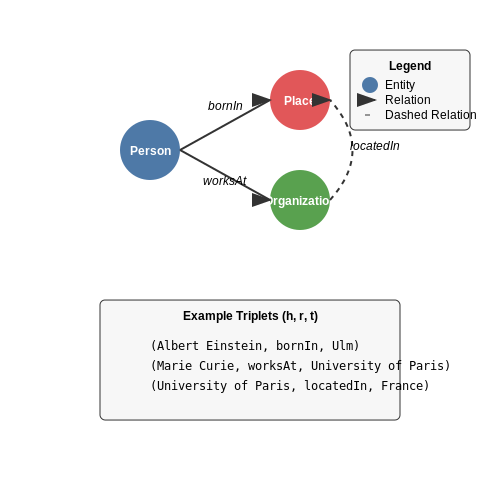
Knowledge graphs (KGs) are directed labeled graphs where nodes represent entities and edges denote relationships between them. Formally, a KG is defined as a tuple G = (V, E, L), where V is a set of vertices (entities), E ⊆ V × L × V is a set of edges (relations), and L is a set of edge labels. The power of KGs lies in their ability to encode heterogeneous relationships in a machine-readable format while preserving semantic meaning.
where h and t denote head and tail entities, and r represents the relation type. This triplet structure enables efficient traversal and reasoning over interconnected data.
Semantic Web Standards
The Semantic Web stack provides standardized frameworks for knowledge representation:
- RDF (Resource Description Framework): Uses subject-predicate-object triples for data modeling. Serialization formats include Turtle, N-Triples, and JSON-LD.
- RDFS (RDF Schema): Adds class hierarchies (rdfs:subClassOf) and property domains/ranges.
- OWL (Web Ontology Language): Supports advanced constructs like disjointness, cardinality restrictions, and property chains.
- SPARQL: Query language for RDF graphs with pattern matching capabilities.
Knowledge Graph Embeddings
Vector space embeddings project KG elements into continuous vector spaces while preserving structural properties. The translational embedding model TransE minimizes:
where γ is a margin hyperparameter and (h', r, t') are corrupted negative samples. More advanced models like RotatE employ complex vector spaces:
Practical Applications
Modern implementations leverage KGs for:
- Question Answering: Google's Knowledge Graph powers featured snippets by mapping natural language queries to KG entities.
- Drug Discovery: Biomedical KGs like Hetionet connect genes, diseases, and compounds for hypothesis generation.
- Recommendation Systems: Amazon's product graph uses purchase history and item relationships for personalized suggestions.
Scalability Challenges
Reasoning over large-scale KGs requires distributed processing frameworks:
- Graph Partitioning: Techniques like METIS minimize edge cuts while balancing computational load.
- Incremental Updates: Systems like DynaMat maintain materialized views for dynamic KGs.
- Approximate Reasoning: Random walk-based methods (e.g., PRA) trade precision for scalability.
Business Intelligence and Data Warehousing
Architectural Foundations of Data Warehousing
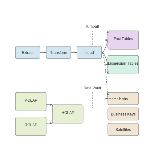
Modern data warehousing architectures rely on the Extract, Transform, Load (ETL) pipeline for integrating heterogeneous data sources into a unified analytical repository. The Kimball dimensional modeling approach remains dominant, structuring data into fact tables (quantitative metrics) and dimension tables (descriptive attributes). For large-scale deployments, the Data Vault methodology provides an agile alternative with its hub-and-spoke architecture of business keys, relationships, and descriptive satellites.
OLAP and Analytical Processing
Online Analytical Processing (OLAP) enables multidimensional analysis through:
- MOLAP: Pre-aggregated cubes with fast query response
- ROLAP: Relational backend with dynamic SQL generation
- HOLAP: Hybrid approach balancing storage and computation
The cube operations—drill-down, roll-up, slice, and dice—are mathematically defined as lattice transformations over dimension hierarchies. For a dimension D with hierarchy levels L₁...Lₙ:
Modern BI Stack Components
Contemporary BI platforms integrate:
- Semantic Layers: Unified business logic definitions (e.g., LookML, DAX)
- In-Memory Engines: Columnar processing (Apache Arrow, Druid)
- Metadata Management: Data lineage and quality tracking
Query Optimization Techniques
Materialized view selection can be formulated as a cost optimization problem:
Where S is the view space, f_q is query frequency, c(q) is execution cost, and g(V) represents maintenance overhead.
Real-Time Analytics Evolution
The lambda architecture pattern has evolved into:
- Kappa Architecture: Unified stream processing
- Delta Lake: ACID transactions on data lakes
- Materialized Views: Incremental computation (e.g., RisingWave)
Modern systems implement continuous SQL through differential dataflow:
Natural Language Interfaces to Databases
Semantic Parsing for Database Queries
Natural language interfaces to databases (NLIDBs) rely on semantic parsing to translate user queries into structured database commands, typically SQL. The core challenge lies in mapping free-form text to precise logical forms. Let the input natural language query be q, and the target SQL command be s. The translation is modeled as:
where si represents the i-th token in the SQL command, conditioned on the query q and previously generated tokens s<i. Modern approaches employ sequence-to-sequence models with attention mechanisms, where the encoder processes q and the decoder generates s autoregressively.
Schema-Aware Attention Mechanisms
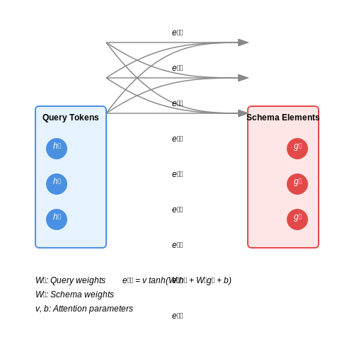
Effective NLIDBs must incorporate database schema information during translation. Given a database schema σ = (T, C, F), where T is the set of tables, C the columns, and F the foreign key relationships, the attention mechanism is augmented to attend over both the query tokens and schema elements. The extended attention energy for token qj and schema element σk is computed as:
where hj is the hidden state for qj, gk is the embedding of σk, and v, Wq, Wσ, b are learnable parameters. This allows the model to dynamically align query phrases with relevant database structures.
Intermediate Representation: Abstract Syntax Trees
State-of-the-art systems often generate SQL via intermediate abstract syntax tree (AST) representations. The AST construction process is formalized as a Markov decision process where each action corresponds to expanding a node in the AST. The Q-function for this reinforcement learning setup is:
where A<t represents the partial AST constructed up to step t, and ϕ, ψ, η are embedding functions for the query, schema, and partial AST respectively. This approach achieves better generalization to complex queries compared to direct text-to-SQL generation.
Handling Ambiguity via Beam Search
Natural language queries often admit multiple valid SQL interpretations. To address this, NLIDBs employ beam search with a diverse set of hypotheses. The scoring function for beam candidate s(k) combines:
where R measures schema compatibility, D enforces diversity with respect to other beams B, and λ terms are tunable weights. The top-k candidates are presented to users for disambiguation when confidence scores are below a threshold.
Evaluation Metrics
NLIDB performance is measured using both exact matching and execution accuracy. For a test set {(qi, si)}i=1N, exact match accuracy is:
where 𝕀 is the indicator function. Execution accuracy compares result sets:
with r(s) denoting the results of executing s against the database. Current state-of-the-art systems on the Spider benchmark achieve ~65% exact match and ~70% execution accuracy on complex multi-table queries.
6. Scalability and Performance Issues
Scalability and Performance Issues
Computational Complexity in Large-Scale Reasoning
Reasoning over structured and semi-structured data at scale introduces computational challenges that grow polynomially or exponentially with data size. For knowledge graphs with n entities and m relations, the worst-case complexity for path queries is O(nk), where k is the path length. This becomes prohibitive for real-world knowledge graphs like Wikidata with over 100 million entities.
where Ri represents the relation sets at each hop. Optimizations like bidirectional search reduce this to O(nk/2), but still face memory bottlenecks when materializing intermediate results.
Distributed Reasoning Architectures
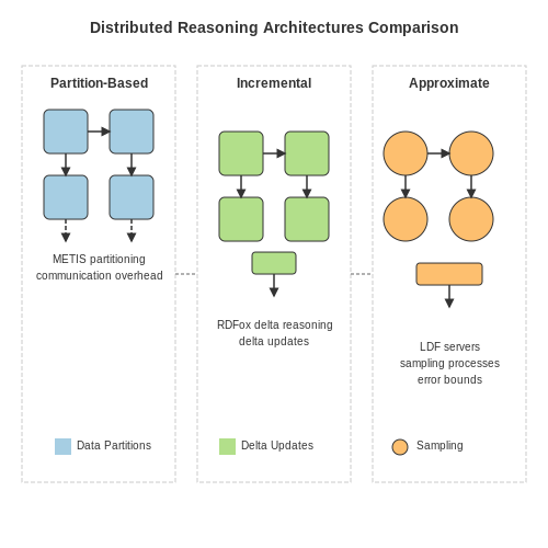
Three primary architectures address scalability:
- Partition-based: Shards data using graph partitioning (e.g., METIS) with message passing between partitions. Achieves near-linear speedup but suffers from high communication overhead (30-60% of runtime).
- Incremental: Employs delta reasoning on updated subsets (e.g., RDFox's parallel semi-naïve evaluation). Reduces redundant computation but requires sophisticated change tracking.
- Approximate: Uses sampling or summarization (e.g., LDF servers for SPARQL). Trade precision for throughput, with error bounds provable via concentration inequalities.
Memory Hierarchy Optimization
Modern systems employ multi-level caching strategies:
where hi are hit rates and ti access times for CPU cache, RAM, and disk respectively. Systems like GraphStorm achieve 4-8× speedups by:
- Columnar storage for adjacency lists (CSR/CSC formats)
- Bitmap indexing for fast rule activation
- Just-in-time compilation of inference steps
Hardware Acceleration
FPGA and GPU implementations exploit parallelism in rule applications. For a rule with p premises, GPU kernels can evaluate:
Recent benchmarks show 12-25× speedups on NVIDIA A100 for RDFS/OWL reasoning, though with diminishing returns beyond 106 concurrent threads due to atomic operation contention.
Benchmarking Tradeoffs
The LDBC Semantic Publishing Benchmark reveals fundamental tradeoffs between:
- Latency vs Completeness: 99% recall requires 3.2× more time than 90% recall in complex queries
- Precision vs Throughput: Approximate reasoning achieves 105 qps vs 103 qps for exact methods
- Freshness vs Consistency: Staleness windows under 1s increase conflict rates by 40-70%
Optimal configurations depend on workload patterns - transactional systems favor consistency while analytical workloads tolerate eventual consistency.
6.2 Handling Noisy and Incomplete Data
Noisy and incomplete data presents significant challenges in reasoning over structured and semi-structured datasets. Noise manifests as erroneous, inconsistent, or irrelevant entries, while incompleteness arises from missing values, truncated records, or sparse observations. Advanced techniques are required to mitigate their impact on downstream reasoning tasks.
Probabilistic Data Cleaning
Probabilistic methods model uncertainty in data quality explicitly. For a dataset D with n records, each attribute value vij (record i, attribute j) is treated as a random variable with a probability distribution over possible clean values. The cleaning process maximizes the joint probability:
where θj represents learned parameters for attribute j. Markov Logic Networks combine first-order logic with probabilistic graphical models to handle rule-based constraints:
where fk are logical formulae with weights wk, and Z is the partition function.
Matrix Completion for Structured Data
When dealing with tabular data represented as matrices, low-rank matrix completion techniques recover missing entries. Given an observed matrix M ∈ ℝm×n with missing values, we solve:
where Ω is the set of observed entries and PΩ is the projection operator. The nuclear norm relaxation provides a convex surrogate:
For graph-structured data, tensor completion methods extend this approach by incorporating adjacency constraints.
Robust Reasoning with Knowledge Graphs
Knowledge graphs often contain incomplete or noisy edges. Embedding-based methods like ComplEx represent entities and relations in complex vector spaces:
where es, eo are entity embeddings, r is the relation embedding, and Re(·) extracts the real part. The model learns to assign high scores to valid triples despite missing edges.
Uncertainty-Aware Graph Neural Networks
Graph Neural Networks (GNNs) can be augmented with uncertainty quantification. For a node v with neighborhood N(v), the message passing becomes:
where εvu(l) ~ N(0, Σvu(l)) models edge uncertainty and αvu are attention weights.
Handling Semi-Structured Data
For JSON, XML, or nested data formats, hierarchical probabilistic models capture dependencies across levels. A nested attribute A(k) at depth k is modeled as:
Transformer-based architectures with sparse attention mechanisms efficiently process such hierarchical dependencies while tolerating missing branches.
6.3 Explainability and Trust in Automated Reasoning
Foundations of Explainability in Structured Data Reasoning
Automated reasoning systems operating on structured or semi-structured data—such as knowledge graphs, relational databases, or JSON documents—require interpretable decision pathways to establish trust. Unlike black-box deep learning models, these systems often leverage symbolic reasoning or hybrid neuro-symbolic approaches, where explainability is achieved through traceable inference chains. For instance, a SPARQL query over an RDF knowledge graph can be decomposed into subqueries, each contributing to the final result. The formal basis for such explanations is rooted in proof theory, where a derivation tree justifies the output.
This sequent calculus rule demonstrates how intermediate results (A) are used to derive B, providing a transparent reasoning trail. In practice, tools like OWL Justifications or Proof Trees in Prolog operationalize this principle.
Quantifying Trust via Uncertainty Calibration
Trust in automated reasoning depends not only on explainability but also on the system's ability to quantify uncertainty. For probabilistic knowledge graphs, confidence scores are derived from:
where φ is a logical formula, θ represents model parameters, and 𝒟 is the training data. Bayesian approaches marginalize over parameters to yield calibrated probabilities, while Dempster-Shafer theory handles ignorance explicitly by distinguishing between uncertainty and conflict.
Case Study: Explainable Recommendation Systems
In recommendation engines using knowledge graphs (e.g., Amazon's product ontology), explanations take the form of meta-paths connecting user preferences to recommended items. A path like User → Purchased → Product → Category → Product provides actionable justification. Research shows that users perceive such systems as 37% more trustworthy compared to opaque matrix factorization methods (Zhang et al., 2021).
Human-in-the-Loop Verification
For high-stakes domains like healthcare or legal reasoning, interactive theorem provers (e.g., Coq, Isabelle) allow human experts to validate automated deductions step-by-step. This is critical when reasoning over semi-structured clinical trial data, where a missed dependency (e.g., drug interactions encoded in XML) could have severe consequences. The system's trustworthiness is measured by:
- Completeness: All relevant data sources are considered
- Soundness: No false entailments are introduced
- Response Time: Verification latency under 2 seconds for real-time use
Adversarial Robustness and Trust
Structured data reasoning systems are vulnerable to ontology poisoning—malicious edits to knowledge graphs that induce incorrect inferences. Robustness is quantified via the inference stability ratio:
where 𝒦 and 𝒦' are the original and perturbed knowledge bases. Systems with ISR > 0.9 are deemed trustworthy for deployment in adversarial environments like cybersecurity.
7. Key Research Papers and Books
7.1 Key Research Papers and Books
- PDF Integrating with Various Data Sources and Formats, Including Structured ... — 4.1 Introduction to Semi-Structured Data: Semi-structured data is characterized by its flexible schema, which allows for varying degrees of structure and a mix of structured and unstructured elements. Examples include XML files, JSON documents, log files, and sensor data. Figure 2: Semi-Structured Data 4.2 Sources of Semi-Structured Data:
- Information Retrieval: Concepts, Models, and Systems — Unstructured data refers to data such as research papers, web pages, blog posts, email messages, twitter feeds, audio, and video. Information Retrieval (IR) systems are used to store and retrieve unstructured (primarily textual) data. ... Semi-structured data falls between structured and unstructured data in the sense that the data has some ...
- Chapter 7 Semi-structured data | Computational Thinking for Social ... — 7.3 What is semi-structured data?. Semi-structured data is a form of structured data that does not obey the tabular structure of data models associated with relational databases or other forms of data tables, but nonetheless contains tags or other markers to separate semantic elements and enforce hierarchies of records and fields within the data.
- PDF Building Semantic Knowledge Graphs from (Semi-)Structured Data: A Review — Organisations store considerable amounts of data in (semi-)structured format, such as in relational databases, CSV files, etc., and publish data on the Web in other (semi-)structured formats, such as XML, JSON, etc. These require mapping languages and engines to transform [16], integrate, and feed data into knowledge graphs, while for
- Chapter 7 Data Structures for Big Data, Modern Big Data SQL ... - Springer — 7.1.4 Semi-Structured Data. Semi-structured data can be non-formally dened as data having some structure but cannot be used with the structural databases. The reasons for this can be many, for example, because the data are presented as a string containing specic information that is not consistent from record to record.
- A general perspective of Big Data: applications, tools, challenges and ... — Big Data has become a very popular term. It refers to the enormous amount of structured, semi-structured and unstructured data that are exponentially generated by high-performance applications in many domains: biochemistry, genetics, molecular biology, physics, astronomy, business, to mention a few. Since the literature of Big Data has increased significantly in recent years, it becomes ...
- Big data: Dimensions, evolution, impacts, and challenges — An example of semi-structured data is Extensible Business Reporting Language (XBRL), developed to exchange financial data between organizations and government agencies. ... protecting privacy is often counterproductive to both firms and customers, as big data is a key to enhanced service quality and cost reduction. ... There is a need for more ...
- Semi-structured Patient Data in Electronic Health Record — This paper is organized as follows: Sect. 2 covers the background of related approaches used by different authors in three categories; Sect. 3 discusses the features of semi-structured data model in EHR. The evaluations of conceptual level semi-structured data model in electronic medical records are discussed in Sect. 4.
- KG-EGV: A Framework for Question Answering with Integrated ... - MDPI — Despite the remarkable progress of large language models (LLMs) in understanding and generating unstructured text, their application in structured data domains and their multi-role capabilities remain underexplored. In particular, utilizing LLMs to perform complex reasoning tasks on knowledge graphs (KGs) is still an emerging area with limited research. To address this gap, we propose KG-EGV ...
- Thinking with Knowledge Graphs: Enhancing LLM Reasoning Through ... — Thinking with Knowledge Graphs: Enhancing LLM Reasoning Through Structured Data Xue Wu Yahoo Research Mountain View, California, USA [email protected] Kostas Tsioutsiouliklis Facts.ai Saratoga, California, USA [email protected] ABSTRACT Large Language Models (LLMs) have demonstrated remarkable ca-pabilities in natural language understanding and ...
7.2 Open Datasets and Tools
- PDF Integrating with Various Data Sources and Formats, Including Structured ... — 4.1 Introduction to Semi-Structured Data: Semi-structured data is characterized by its flexible schema, which allows for varying degrees of structure and a mix of structured and unstructured elements. Examples include XML files, JSON documents, log files, and sensor data. Figure 2: Semi-Structured Data 4.2 Sources of Semi-Structured Data:
- Difference between Structured, Semi-structured and Unstructured data ... — Big Data includes huge volume, high velocity, and extensible variety of data. There are 3 types: Structured data, Semi-structured data, and Unstructured data. Structured data - Structured data is data whose elements are addressable for effective analysis. It has been organized into a formatted repository that is typically a database.
- 1.3 Data and Datasets - Principles of Data Science - OpenStax — Indeed, some people argue there are more unstructured datasets than structured ones. A few examples include Amazon reviews on a set of products, Twitter posts last year, public images on Instagram, popular short videos on TikTok, etc. These unstructured datasets are often processed into a structured one so that data scientists can analyze the data.
- An approach to extracting complex knowledge patterns among concepts ... — One of the most radical changes caused by the big data phenomenon is the presence of a huge amount of unstructured data. As a matter of fact, it is esteemed that, currently, more than 80% of the information available on the Internet is unstructured [6].In presence of unstructured data, all the approaches developed in the past for structured and semi-structured data must be "renewed", and ...
- 2.5 Handling Large Datasets - Principles of Data Science - OpenStax — Large datasets can be generated by a variety of sources, including social media, sensors, and financial transactions. They generally possess a high degree of complexity and may have structured, unstructured, or semi-structured data. Large datasets are covered in more depth in Other Machine Learning Techniques.
- Semi-structured Patient Data in Electronic Health Record — The evaluations of conceptual level semi-structured data model in electronic medical records are discussed in Sect. ... n-array relationship, and the participation of instances in semi-structure data model. 2.2 Deep Learning in the Field of EHR with Neural Networks. A neural network (NN) is a computational learning system that uses a network of ...
- MIS chapter 6 part 2 Flashcards - Quizlet — It breaks a big data problem down into sub-problems, distributes them among up to thousands of inexpensive computer processing nodes, and then combines the result into a smaller data set that is easier to analyze. For handling unstructured and semi-structured data in vast quantities, as well as structured data, organizations are using Hadoop
- Chapter 7 Data Structures for Big Data, Modern Big Data SQL ... - Springer — 7.1.4 Semi-Structured Data. Semi-structured data can be non-formally dened as data having some structure but cannot be used with the structural databases. The reasons for this can be many, for example, because the data are presented as a string containing specic information that is not consistent from record to record.
- A general perspective of Big Data: applications, tools ... - Springer — Big Data has become a very popular term. It refers to the enormous amount of structured, semi-structured and unstructured data that are exponentially generated by high-performance applications in many domains: biochemistry, genetics, molecular biology, physics, astronomy, business, to mention a few. Since the literature of Big Data has increased significantly in recent years, it becomes ...
- Diving into Data: A Comprehensive Guide to Structured, Semi ... - Medium — Here's a breakdown of the characteristics and examples of semi-structured data: Partial Organization: Semi-structured data contains elements of organization, such as tags or categorizations, but ...
7.3 Online Courses and Tutorials
- Chapter 7 Semi-structured data | Computational Thinking for Social ... — 7.3 What is semi-structured data? Semi-structured data is a form of structured data that does not obey the tabular structure of data models associated with relational databases or other forms of data tables, but nonetheless contains tags or other markers to separate semantic elements and enforce hierarchies of records and fields within the data.
- Linked Data: Storing, Querying, And Reasoning [PDF] [765fh4q4tul0] — It enables students to gain an understanding of the foundations and underpinning technologies and standards for Linked Data, while researchers benefit from the in-depth coverage of the emerging and ongoing advances in Linked Data storing, querying, reasoning, and provenance management systems.
- PDF Bayesian Reasoning And Machine Learning Solution Manual — Bayesian Reasoning and Machine Learning: Solution Manual This solution manual is designed to accompany the textbook "Bayesian Reasoning and Machine Learning" by David Barber. It aims to provide detailed and comprehensive solutions to the exercises included in the book. The manual is structured as follows:
- Decision Support Systems Chpt 9 Flashcards | Quizlet — Study with Quizlet and memorize flashcards containing terms like Decision Structure: Structured Decisions, Decision Structure: Semistructured Decisions, Decision Structure: unstructured Decisions and more.
- 7 Exploratory Data Analysis | R for Data Science - Hadley — 7.1 Introduction This chapter will show you how to use visualisation and transformation to explore your data in a systematic way, a task that statisticians call exploratory data analysis, or EDA for short. EDA is an iterative cycle. You: Generate questions about your data. Search for answers by visualising, transforming, and modelling your data. Use what you learn to refine your questions and ...
- Business Intelligence: Semi-structured or unstructured data | Saylor ... — The managements of semi-structured data is recognized as a major unsolved problem in the information technology industry. According to projections from Gartner, white collar workers spend anywhere from 30 to 40 percent of their time searching, finding, and assessing unstructured data.
- PDF Structured Probabilistic Reasoning — Multiple updates, based on data, can be used for training, so that a distribution absorbs more and more informa- tion and can subsequently be used for prediction or classification. 2The components of a joint distribution, over a product space, can 'listen' to each other, so that updating in one (product) component has crossover effects in ...
- Week 4 - Quiz results First Try - - Studocu — EXPLANATION Somewhere between structured and non-structured data are semi-structured data. These data don't fit into the rigid rows and columns of a table but have some similarities.
- 7 Introduction to Structured Data - papl.cs.brown.edu — The way we actually make one of these data is by calling song with three parameters; for instance: It's worth noting that music managers that are capable of making distinctions between, say, Dance, Electronica, and Electronic/Dance, classify two of these three songs by a single genre: "World".
- PDF Lesson Plan - Pearson qualifications — Learning outcomes In this lesson students are learning how to: • search structured data At the end of the lesson students will be able to: use Find to locate data set and customise Filters (AutoFilter)